Deep Learning - Loss Functions

一、损失函数概述

大多数深度学习算法都会涉及某种形式的优化，所谓优化指的是改变 \(x\) 以最小化或最大化某个函数 \(f(x)\) 的任务，我们通常以最小化 \(f(x)\) 指代大多数最优化问题。

在机器学习中，损失函数是代价函数的一部分，而代价函数是目标函数的一种类型。

• 损失函数（loss function）: 用于定义单个训练样本预测值与真实值之间的误差
• 代价函数（cost function）: 用于定义单个批次/整个训练集样本预测值与真实值之间的累计误差。
• 目标函数（objective function）: 泛指任意可以被优化的函数。

损失函数定义：损失函数是用来量化模型预测和真实标签之间差异的一个非负实数函数。

损失函数大致可分为两种：回归损失（针对连续型变量）和分类损失（针对离散型变量），常用的减少损失函数的优化算法是“梯度下降法”（Gradient Descent）。

二、分类损失

交叉熵损失(Cross-Entropy Loss) 又称为对数似然损失(Log-likelihood Loss)、对数损失，二分类时还可称之为逻辑斯谛回归损失(Logistic Loss)。

2.1 熵Entropy

1，信息量

信息论中，信息量(自信息 self-information) 的表示方式。 在本文中，我们总是用 \(\text{log}\) 来表示自然对数，其底数为 \(e\)。

\[I(x_j) = -\log (p(x_j))\]

• \(x_j\)：表示一个事件
• \(p(x_j)\)：表示事件 \(x_j\) 发生的概率
• \(I(x_j)\)：信息量，\(x_j\) 越不可能发生时，它一旦发生后的信息量就越大

2，熵

信息量只处理单个的输出。我们可以用熵（entropy）来对整个概率分布中的不确定性总量进行量化:

\[H(p) = - \sum_j^n p(x_j) \log (p(x_j))\]

3，相对熵(KL散度)

相对熵又称KL散度，如果对于同一个随机变量 \(x\) 有两个单独的概率分布 \(P(x)\) 和 \(Q(x)\)，则可以使用 KL 散度（Kullback-Leibler (KL) divergence）来衡量这两个分布的差异，这个相当于信息论范畴的均方差。

KL散度的计算公式：

\[D_{KL}(p||q)=\sum_{j=1}^m p(x_j) \log {p(x_j) \over q(x_j)}\]

\(m\) 为事件的所有可能性（分类任务中对应类别数目）。\(D\) 的值越小，表示 \(q\) 分布和 \(p\) 分布越接近。

4，交叉熵

把上述交叉熵公式变形：

\[\begin{aligned} D_{KL}(p||q)&=\sum_{j=1}^m p(x_j) \log {p(x_j)} - \sum_{j=1}^m p(x_j) \log q(x_j) \\\ &=- H(p(x)) + H(p,q) \end{aligned}\]

等式的前一部分恰巧就是 \(p\) 的熵，等式的后一部分，就是交叉熵（机器学习中 \(p\) 表示真实分布（目标分布），\(q\) 表示预测分布）:

\[H(p,q) =- \sum_{j=1}^m p(x_j) \log q(x_j)\]

在机器学习中，我们需要评估标签值 \(y\) 和预测值 \(a\) 之间的差距熵（即两个概率分布之间的相似性），使用 KL 散度 $$D_{KL}(y

a)\(即可，但因为样本标签值的分布通常是固定的，即\)H(a)$$ 不变。因此，为了计算方便，在优化过程中，只需要关注交叉熵就可以了。所以，在机器学习中一般直接用交叉熵做损失函数来评估模型。

\[loss = -\sum_{j = 1}^{m}y_{j}\text{log}(a_{j})\]

2.2，交叉熵二分类可视化

有一类特殊问题，就是事件只有两种情况发生的可能，比如“是狗”和“不是狗”，称为 \(0/1\) 分类或二分类。对于这类问题，由于 \(m=2，y_1=1-y_2，a_1=1-a_2\)，所以二分类问题的单个样本的交叉熵可以简化为：

\[loss =-[y \log a + (1-y) \log (1-a)]\]

把二分类的交叉熵公式 4 分解开两种情况：

• 当 \(y=1\) 时，即标签值是 \(1\) ，是个正例，加号后面的项为: \(loss = -\log(a)\)
• 当 \(y=0\) 时，即标签值是 \(0\)，是个反例，加号前面的项为 \(0\): \(loss = -\log (1-a)\)

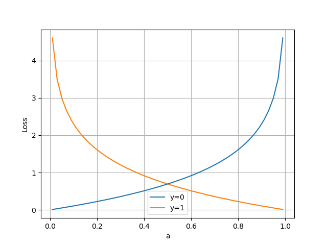
横坐标是预测输出，纵坐标是损失函数值。\(y=1\) 意味着当前样本标签值是1，当预测输出越接近1时，损失函数值越小，训练结果越准确。当预测输出越接近0时，损失函数值越大，训练结果越糟糕。此时，损失函数值如下图所示。

2.4，为什么不能使用均方差做为分类问题的损失函数？

原因1：凸函数

凸函数的优点是：无论初始参数如何，梯度下降（或其他优化算法）都能保证收敛到全局最优解。

MSE是预测值\(\hat{y}_i\)的二次函数（平方项），其二阶导数为常数2，始终为正，因此，MSE 是凸函数。

如果模型输出是线性的MSE 是凸的。但在分类问题中，模型通常包含非线性激活函数（如 sigmoid 或 softmax）以输出概率，MSE 的损失函数相对于模型参数不再是凸函数。具体来说，sigmoid 或 softmax 的非线性变换使得损失函数的二阶导数（Hessian 矩阵）不再始终正定，导致损失函数可能有多个局部极小值（non-convex）。

原因2：分类边界

交叉熵通过放大错误预测的惩罚（对数形式），推动模型学习清晰的分类边界。MSE 可能导致模型在“数值上接近”但分类错误的区域停留（例如，预测 0.51 而不是 0.99）。

原因3：鲁棒性：

交叉熵对概率值的约束（通过 sigmoid 或 softmax）确保输出在 [0, 1] 区间，且多分类中概率和为 1，符合概率分布的要求。MSE 不保证这种约束，可能导致不合理的输出（如负值或大于 1）

三、回归损失

与分类问题不同，回归问题解决的是对具体数值的预测。解决回归问题的神经网络一般只有只有一个输出节点，这个节点的输出值就是预测值。

回归问题的一个基本概念是残差或称为预测误差，用于衡量模型预测值与真实标记的靠近程度。假设回归问题中对应于第 \(i\) 个输入特征 \(x_i\) 的标签为 \(y^i = (y_1,y_2,...,y_M)^{\top}\)，\(M\) 为标记向量总维度，则 \(l_{t}^{i}\) 即表示样本 \(i\) 上神经网络的回归预测值 (\(y^i\)) 与其样本标签值在第 \(t\) 维的预测误差(亦称残差):

\[l_{t}^{i} = y_{t}^{i} - \hat{y}_{t}^{i}\]

常用的两种损失函数为 \(\text{MAE}\)（也叫 L1 损失） 和 \(\text{MSE}\) 损失函数（也叫 L2 损失）。

3.1 MAE 损失

平均绝对误差（Mean Absolute Error，MAE）是用于回归模型的最简单但最强大的损失函数之一。

因为存在离群值（与其余数据差异很大的值），所以回归问题可能具有本质上不是严格高斯分布的变量。 在这种情况下，平均绝对误差将是一个理想的选择，因为它没有考虑异常值的方向（不切实际的高正值或负值）。

顾名思义，MAE 是目标值和预测值之差的绝对值之和。\(n\) 是数据集中数据点的总数，其公式如下:

\[\text{MAE loss} = \frac{1}{n}\sum_{i=1}^{N}\sum_{t=1}^{M} |y_{t}^{i} - \hat{y}_{t}^{i}|\]

3.2 MSE 损失

均方误差（Mean Square Error, MSE）几乎是每个数据科学家在回归损失函数方面的偏好，这是因为大多数变量都可以建模为高斯分布。均方误差计算方法是求预测值与真实值之间距离的平方和。预测值和真实值越接近，两者的均方差就越小。公式如下:

\[\text{MSE loss} = \frac{1}{n}\sum_{i=1}^{N}\sum_{t=1}^{M} (y_{t}^{i} - \hat{y}_{t}^{i})^2\]

3.3 Huber 损失

MAE 和 MSE 损失之间的比较产生以下结果：

1. MAE 损失比 MSE 损失更稳健。仔细查看公式，可以观察到如果预测值和实际值之间的差异很大，与 MAE 相比，MSE 损失会放大效果。 由于 MSE 会屈服于异常值，因此 MAE 损失函数是更稳健的损失函数。

2. MAE 损失不如 MSE 损失稳定。由于 MAE 损失处理的是距离差异，因此一个小的水平变化都可能导致回归线波动很大。在多次迭代中发生的影响将导致迭代之间的斜率发生显著变化。总结就是，MSE 可以确保回归线轻微移动以对数据点进行小幅调整。
3. MAE 损失更新的梯度始终相同。即使对于很小的损失值，梯度也很大。这样不利于模型的学习。为了解决这个缺陷，我们可以使用变化的学习率，在损失接近最小值时降低学习率。
4. MSE 损失的梯度随损失增大而增大，而损失趋于0时则会减小。其使用固定的学习率也可以有效收敛。

Huber Loss 结合了 MAE 的稳健性和 MSE 的稳定性，本质上是 MAE 和 MSE 损失中最好的。对于大误差，它是线性的，对于小误差，它本质上是二次的。

Huber Loss 的特征在于参数 \(\delta\)。当 $$

y − \hat{y}

$$ 小于一个事先指定的值 $\delta $ 时，变为平方损失，大于 $\delta $ 时，则变成类似于绝对值损失，因此其是比较robust 的损失函数。其定义如下:

\[\text{Huber loss} = \left \lbrace \begin{matrix} \frac12[y_{t}^{i} - \hat{y}_{t}^{i}]^2 & |y_{t}^{i} - \hat{y}_{t}^{i}| \leq \delta \\ \delta|y_{t}^{i} - \hat{y}_{t}^{i}| - \frac12\delta^2 & |y_{t}^{i} - \hat{y}_{t}^{i})| > \delta \end{matrix}\right.\]

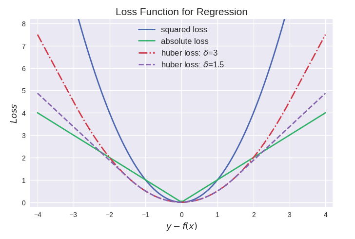
三种回归损失函数的曲线图比较如下：

四、其他损失函数

4.1 Focal 损失

通过调节难易样本权重解决数据倾斜问题，适用于长尾分布场景的二分类问题：

\[Focal = -\alpha_t(1-p_t)^{\gamma}log(p_t)\]

其中：

• \(p_t\)是模型对真实类别的预测概率：\(p_t=\left\{ \begin{array}{l} p ,正样本\\ 1-p,负样本 \end{array} \right.\)
• \(\alpha\in[0,1]\)：类别平衡因子，通常为稀有类别分配更高权重，通常0.25。
• \(\gamma\geq 1\)： 困难样本聚焦参数，调整难易样本的权重比例，通常2。

4.2 Tweedie 损失

Tweedie loss函数是一种基于 Tweedie 分布的回归损失函数，广泛应用于处理 零膨胀（zero-inflated） 和 右偏（right-skewed） 数据

\[L(y, \hat{y}; p) = \left\{ \begin{array}{ll} 2 \left[ \frac{y^{2-p}}{(1-p)(2-p)} - \frac{y \hat{y}^{1-p}}{1-p} + \frac{\hat{y}^{2-p}}{2-p} \right] & \text{if } y > 0 \\ 2 \frac{\hat{y}^{2-p}}{2-p} & \text{if } y = 0 \end{array} \right\}\]

• \(y\)：真实值（目标变量）

• \(\hat{y}\)：预测值，需确保 \(\hat{y}>0\)
• \(p\)：方差功率参数，控制分布的“混合”程度（默认 1.5）
• 当\(y=0\)时，损失仅惩罚预测的非零值，以鼓励模型在零值处输出零。

五、代码实现

#手写版本
def mae(true, pred):
    loss = np.abs(true - pred)
    return np.mean(loss)

def mse(true, pred):
    loss = (true - pred)**2
    return np.mean(loss)

def huber(true, pred, delta):
    
    loss = np.where(np.abs(true-pred) < delta , 0.5*((true-pred)**2),delta*np.abs(true - pred) - 0.5*(delta**2))
    
    return np.mean(loss)

def bce(true, pred):
    pred_prob = 1 / (1 + np.exp(-pred))
    
    epsilon = 1e-15
    pred_prob = np.clip(pred_prob, epsilon, 1 - epsilon)
    
    loss = -(true * np.log(pred_prob) + (1 - true) * np.log(1 - pred_prob))
    return np.mean(loss)

def cross_entropy(y_true, y_pred):
    """
    计算交叉熵损失（需配合 Softmax 使用），带数值稳定处理
    :param y_true: one-hot 编码的真实标签，形状 (n_samples, n_classes)
    :param y_pred: 模型输出的 logits，形状 (n_samples, n_classes)
    :return: 标量损失值
    """
    # 数值稳定处理：减去最大值防止指数爆炸
    exps = np.exp(y_pred - np.max(y_pred, axis=1, keepdims=True))
    softmax_output = exps / np.sum(exps, axis=1, keepdims=True)
    # 避免 log(0) 导致数值问题
    epsilon = 1e-7
    clipped = np.clip(softmax_output, epsilon, 1 - epsilon)
    # 只计算真实类别对应的损失
    n_samples = y_true.shape[0]
    log_likelihood = -np.log(clipped[range(n_samples), y_true.argmax(axis=1)])
    return np.mean(log_likelihood)

def kl_divergence(p, q):
    """
    计算两个离散分布的KL散度
    :param p: 真实概率分布，形状 (n_classes, )
    :param q: 预测概率分布，形状 (n_classes, )
    :return: 标量散度值
    """
    # 过滤零元素避免数值问题
    mask = (p != 0)
    p = p[mask]
    q = q[mask]
    return np.sum(p * np.log(p / q))

def focal_loss(y_true, y_pred, alpha=0.25, gamma=2.0):
    """
    计算二分类Focal Loss
    :param y_true: 真实标签 (n_samples, )
    :param y_pred: 预测概率 (n_samples, )
    :param alpha: 类别平衡因子
    :param gamma: 困难样本聚焦参数
    :return: 标量损失值
    """
    epsilon = 1e-7
    y_pred = np.clip(y_pred, epsilon, 1 - epsilon)
    p_t = y_true * y_pred + (1 - y_true) * (1 - y_pred)
    alpha_factor = y_true * alpha + (1 - y_true) * (1 - alpha)
    loss = -alpha_factor * (1 - p_t) ** gamma * np.log(p_t)
    return np.mean(loss)


# 示例用法（处理文本分类中的长尾分布）
y_true = np.array([1, 0, 1, 1, 0])  # 多数类别为1
y_pred = np.array([0.9, 0.2, 0.8, 0.7, 0.1])
print(f"Focal Loss: {focal_loss(y_true, y_pred):.4f}")  # 输出约0.032
#pytorch形式
mae_loss = nn.L1Loss()
mse_loss = nn.MSELoss()
huber_loss =n n.HuberLoss(delta=1.0)
cross_entropy_loss = nn.CrossEntropyLoss(weight=weights)
bce_with_logits_loss = nn.BCEWithLogitsLoss()

1. Overview of Loss Functions

Most deep learning algorithms involve some form of optimization. Optimization means changing \(x\) in order to minimize or maximize some function \(f(x)\); we usually refer to most optimization problems as minimizing \(f(x)\).

In machine learning, the loss function is part of the cost function, and the cost function is one type of objective function.

• Loss function: defines the error between the predicted value and the true value for a single training sample.
• Cost function: defines the accumulated error between predicted and true values over a single batch or the whole training set.
• Objective function: a general term for any function that can be optimized.

Definition of loss function: a loss function is a non-negative real-valued function used to quantify the difference between a model’s prediction and the true label.

Loss functions can be roughly divided into two kinds: regression losses (for continuous variables) and classification losses (for discrete variables). The most commonly used optimization algorithm for reducing the loss is gradient descent.

2. Classification Losses

The cross-entropy loss (Cross-Entropy Loss) is also called the log-likelihood loss or log loss, and in the binary case it can also be called the logistic loss (Logistic Loss).

2.1 Entropy

1. Amount of information

In information theory, the amount of information (self-information) is expressed as follows. In this article, \(\text{log}\) always denotes the natural logarithm, whose base is \(e\).

\[I(x_j) = -\log (p(x_j))\]

• \(x_j\): an event
• \(p(x_j)\): the probability that event \(x_j\) occurs
• \(I(x_j)\): the amount of information; the less likely \(x_j\) is, the more information it carries once it happens

2. Entropy

The amount of information only deals with a single outcome. We can use entropy to quantify the total uncertainty in an entire probability distribution:

\[H(p) = - \sum_j^n p(x_j) \log (p(x_j))\]

3. Relative entropy (KL divergence)

Relative entropy, also known as KL divergence, can be used when the same random variable \(x\) has two separate probability distributions \(P(x)\) and \(Q(x)\); the Kullback-Leibler (KL) divergence measures the difference between these two distributions, and is the information-theoretic analogue of mean squared error.

The formula for KL divergence:

\[D_{KL}(p||q)=\sum_{j=1}^m p(x_j) \log {p(x_j) \over q(x_j)}\]

Here \(m\) is the number of all possible events (the number of classes in a classification task). The smaller the value of \(D\), the closer the \(q\) distribution is to the \(p\) distribution.

4. Cross entropy

Rearranging the formula above:

\[\begin{aligned} D_{KL}(p||q)&=\sum_{j=1}^m p(x_j) \log {p(x_j)} - \sum_{j=1}^m p(x_j) \log q(x_j) \\\ &=- H(p(x)) + H(p,q) \end{aligned}\]

The first part of the equation happens to be the entropy of \(p\), and the second part is the cross entropy (in machine learning, \(p\) denotes the true distribution (target distribution) and \(q\) the predicted distribution):

\[H(p,q) =- \sum_{j=1}^m p(x_j) \log q(x_j)\]

In machine learning we need to evaluate the divergence (that is, the similarity between two probability distributions) between the label value \(y\) and the predicted value \(a\), for which the KL divergence $$D_{KL}(y

a)\(suffices. However, because the distribution of the sample labels is usually fixed — that is,\)H(a)$$ is constant — we only need to focus on the cross entropy during optimization for computational convenience. Therefore, in machine learning the cross entropy is generally used directly as the loss function to evaluate the model.

\[loss = -\sum_{j = 1}^{m}y_{j}\text{log}(a_{j})\]

2.2 Visualizing Binary Cross Entropy

There is a special class of problems in which an event has only two possible outcomes, such as “is a dog” and “is not a dog”; these are called \(0/1\) classification or binary classification. For such problems, since \(m=2\), \(y_1=1-y_2\) and \(a_1=1-a_2\), the cross entropy of a single sample in binary classification simplifies to:

\[loss =-[y \log a + (1-y) \log (1-a)]\]

Expanding the binary cross-entropy formula into its two cases:

• When \(y=1\), i.e. the label is \(1\) and the sample is positive, the term after the plus sign gives: \(loss = -\log(a)\)
• When \(y=0\), i.e. the label is \(0\) and the sample is negative, the term before the plus sign is \(0\): \(loss = -\log (1-a)\)

The horizontal axis is the predicted output and the vertical axis is the loss value. With \(y=1\), meaning the current sample label is 1, the closer the predicted output is to 1, the smaller the loss and the more accurate the training result; the closer the predicted output is to 0, the larger the loss and the worse the result. The loss curve is shown below.

2.4 Why Can’t Mean Squared Error Be Used as the Loss for Classification?

Reason 1: Convexity

The advantage of a convex function is that, regardless of the initial parameters, gradient descent (or any other optimizer) is guaranteed to converge to the global optimum.

MSE is a quadratic function of the predicted values \(\hat{y}_i\), and its second derivative is the constant 2, which is always positive; therefore MSE is convex.

If the model output is linear, MSE is convex. But in classification problems the model usually contains nonlinear activations (such as sigmoid or softmax) in order to output probabilities, and the MSE loss is no longer convex with respect to the model parameters. Concretely, the nonlinear transformation of sigmoid or softmax means the second derivative (Hessian matrix) of the loss is no longer always positive definite, so the loss may have multiple local minima (non-convex).

Reason 2: Decision boundary

Cross entropy magnifies the penalty for wrong predictions (through the logarithm), pushing the model to learn a clear decision boundary. MSE may let the model linger in regions that are “numerically close” but misclassified (for example, predicting 0.51 instead of 0.99).

Reason 3: Robustness

The constraints cross entropy imposes on probabilities (through sigmoid or softmax) ensure that outputs lie in the interval [0, 1] and that probabilities sum to 1 in multi-class problems, which matches the requirements of a probability distribution. MSE does not guarantee such constraints and may produce unreasonable outputs (such as negative values or values greater than 1).

3. Regression Losses

Unlike classification problems, regression problems deal with predicting concrete numerical values. A neural network solving a regression problem generally has only one output node, and the output value of that node is the prediction.

A basic concept in regression is the residual, also called the prediction error, which measures how close the model’s prediction is to the true label. Suppose that in a regression problem the label corresponding to the \(i\)-th input feature \(x_i\) is \(y^i = (y_1,y_2,...,y_M)^{\top}\), where \(M\) is the total dimension of the label vector; then \(l_{t}^{i}\) denotes the prediction error (also called residual) of the network’s regression prediction (\(y^i\)) for sample \(i\) against its sample label along the \(t\)-th dimension:

\[l_{t}^{i} = y_{t}^{i} - \hat{y}_{t}^{i}\]

Two commonly used loss functions are the \(\text{MAE}\) (also called L1 loss) and the \(\text{MSE}\) (also called L2 loss).

3.1 MAE Loss

Mean Absolute Error (MAE) is one of the simplest yet most powerful loss functions for regression models.

Because of outliers (values that differ greatly from the rest of the data), a regression problem may involve variables whose underlying distribution is not strictly Gaussian. In that case mean absolute error is an ideal choice, because it does not take the direction of the outlier into account (unrealistically large positive or negative values).

As its name suggests, MAE is the sum of the absolute differences between target and predicted values. With \(n\) the total number of data points in the dataset, its formula is:

\[\text{MAE loss} = \frac{1}{n}\sum_{i=1}^{N}\sum_{t=1}^{M} |y_{t}^{i} - \hat{y}_{t}^{i}|\]

3.2 MSE Loss

Mean Square Error (MSE) is almost every data scientist’s favorite regression loss, because most variables can be modeled as Gaussian distributions. Mean square error computes the sum of the squared distances between predicted and true values. The closer the prediction is to the true value, the smaller the mean square error. The formula is:

\[\text{MSE loss} = \frac{1}{n}\sum_{i=1}^{N}\sum_{t=1}^{M} (y_{t}^{i} - \hat{y}_{t}^{i})^2\]

3.3 Huber Loss

Comparing MAE and MSE leads to the following conclusions:

1. MAE is more robust than MSE. Looking carefully at the formulas, you can observe that when the difference between the predicted and actual value is large, MSE amplifies the effect compared with MAE. Because MSE succumbs to outliers, MAE is the more robust loss function.
2. MAE is less stable than MSE. Because MAE deals with distance differences, even a small horizontal change can make the regression line fluctuate a lot. Effects that occur across many iterations cause significant changes in the slope between iterations. In short, MSE ensures that the regression line moves only slightly to make small adjustments to data points.
3. The gradient of MAE is always the same. Even for very small loss values the gradient is large, which is not conducive to learning. To address this shortcoming we can use a variable learning rate, lowering it as the loss approaches its minimum.
4. The gradient of MSE grows as the loss grows, and shrinks as the loss approaches 0, so a fixed learning rate also converges effectively.

Huber loss combines the robustness of MAE with the stability of MSE; it is essentially the best of both worlds. It is linear for large errors and essentially quadratic for small errors.

Huber loss is characterized by the parameter \(\delta\). When $$

y − \hat{y}

\(is smaller than a pre-specified value\)\delta\(it becomes a squared loss, and when it is larger than\)\delta$$ it becomes similar to an absolute-value loss, which makes it a relatively robust loss function. It is defined as:

\[\text{Huber loss} = \left \lbrace \begin{matrix} \frac12[y_{t}^{i} - \hat{y}_{t}^{i}]^2 & |y_{t}^{i} - \hat{y}_{t}^{i}| \leq \delta \\ \delta|y_{t}^{i} - \hat{y}_{t}^{i}| - \frac12\delta^2 & |y_{t}^{i} - \hat{y}_{t}^{i})| > \delta \end{matrix}\right.\]

A comparison of the curves of the three regression loss functions is shown below:

4. Other Loss Functions

4.1 Focal Loss

It addresses data imbalance by adjusting the weights of easy and hard samples, and is suitable for binary classification problems with long-tailed distributions:

\[Focal = -\alpha_t(1-p_t)^{\gamma}log(p_t)\]

where:

• \(p_t\) is the model’s predicted probability for the true class: \(p_t=\left\{ \begin{array}{l} p ,positive\ sample\\ 1-p,negative\ sample \end{array} \right.\)
• \(\alpha\in[0,1]\): the class balance factor; usually rarer classes get a higher weight, typically 0.25.
• \(\gamma\geq 1\): the hard-sample focusing parameter, which adjusts the weight ratio between hard and easy samples, typically 2.

4.2 Tweedie Loss

The Tweedie loss is a regression loss based on the Tweedie distribution, widely used for zero-inflated and right-skewed data:

\[L(y, \hat{y}; p) = \left\{ \begin{array}{ll} 2 \left[ \frac{y^{2-p}}{(1-p)(2-p)} - \frac{y \hat{y}^{1-p}}{1-p} + \frac{\hat{y}^{2-p}}{2-p} \right] & \text{if } y > 0 \\ 2 \frac{\hat{y}^{2-p}}{2-p} & \text{if } y = 0 \end{array} \right\}\]

• \(y\): the true value (target variable)
• \(\hat{y}\): the predicted value; \(\hat{y}>0\) must hold
• \(p\): the variance power parameter, controlling how “mixed” the distribution is (default 1.5)
• When \(y=0\), the loss only penalizes non-zero predictions, encouraging the model to output zero at zero-valued targets.

5. Code Implementation

# Hand-written versions
def mae(true, pred):
    loss = np.abs(true - pred)
    return np.mean(loss)

def mse(true, pred):
    loss = (true - pred)**2
    return np.mean(loss)

def huber(true, pred, delta):
    
    loss = np.where(np.abs(true-pred) < delta , 0.5*((true-pred)**2),delta*np.abs(true - pred) - 0.5*(delta**2))
    
    return np.mean(loss)

def bce(true, pred):
    pred_prob = 1 / (1 + np.exp(-pred))
    
    epsilon = 1e-15
    pred_prob = np.clip(pred_prob, epsilon, 1 - epsilon)
    
    loss = -(true * np.log(pred_prob) + (1 - true) * np.log(1 - pred_prob))
    return np.mean(loss)

def cross_entropy(y_true, y_pred):
    """
    Compute the cross-entropy loss (to be used together with softmax),
    with numerical stabilization.
    :param y_true: one-hot encoded true labels, shape (n_samples, n_classes)
    :param y_pred: model logits, shape (n_samples, n_classes)
    :return: scalar loss value
    """
    # Numerical stabilization: subtract the max to avoid exponential overflow
    exps = np.exp(y_pred - np.max(y_pred, axis=1, keepdims=True))
    softmax_output = exps / np.sum(exps, axis=1, keepdims=True)
    # Avoid numerical issues caused by log(0)
    epsilon = 1e-7
    clipped = np.clip(softmax_output, epsilon, 1 - epsilon)
    # Only compute the loss for the true class
    n_samples = y_true.shape[0]
    log_likelihood = -np.log(clipped[range(n_samples), y_true.argmax(axis=1)])
    return np.mean(log_likelihood)

def kl_divergence(p, q):
    """
    Compute the KL divergence between two discrete distributions.
    :param p: true probability distribution, shape (n_classes, )
    :param q: predicted probability distribution, shape (n_classes, )
    :return: scalar divergence value
    """
    # Filter out zero elements to avoid numerical issues
    mask = (p != 0)
    p = p[mask]
    q = q[mask]
    return np.sum(p * np.log(p / q))

def focal_loss(y_true, y_pred, alpha=0.25, gamma=2.0):
    """
    Compute the binary Focal Loss.
    :param y_true: true labels (n_samples, )
    :param y_pred: predicted probabilities (n_samples, )
    :param alpha: class balance factor
    :param gamma: hard-sample focusing parameter
    :return: scalar loss value
    """
    epsilon = 1e-7
    y_pred = np.clip(y_pred, epsilon, 1 - epsilon)
    p_t = y_true * y_pred + (1 - y_true) * (1 - y_pred)
    alpha_factor = y_true * alpha + (1 - y_true) * (1 - alpha)
    loss = -alpha_factor * (1 - p_t) ** gamma * np.log(p_t)
    return np.mean(loss)


# Example usage (handling long-tailed distributions in text classification)
y_true = np.array([1, 0, 1, 1, 0])  # the majority class is 1
y_pred = np.array([0.9, 0.2, 0.8, 0.7, 0.1])
print(f"Focal Loss: {focal_loss(y_true, y_pred):.4f}")  # roughly 0.032
# PyTorch versions
mae_loss = nn.L1Loss()
mse_loss = nn.MSELoss()
huber_loss =n n.HuberLoss(delta=1.0)
cross_entropy_loss = nn.CrossEntropyLoss(weight=weights)
bce_with_logits_loss = nn.BCEWithLogitsLoss()