Deep Learning - Normalization Layers

Posted Sep 24, 2023

By Guanlong Ma

38 min read

一、内部协变量转移Internal Covariate Shift

训练深度神经网络的复杂性在于，因为前面的层的参数会发生变化导致每层输入的分布在训练过程中会发生变化。这又导致模型需要需要较低的学习率和非常谨慎的参数初始化策略，从而减慢了训练速度，并且具有饱和非线性的模型训练起来也非常困难。

网络层输入数据分布发生变化的这种现象称为内部协变量转移，BN 就是来解决这个问题。

2.1，如何理解 Internal Covariate Shift

在深度神经网络训练的过程中，由于网络中参数变化而引起网络中间层数据分布发生变化的这一过程被称在论文中称之为内部协变量偏移（Internal Covariate Shift）。

那么，为什么网络中间层数据分布会发生变化呢？

在深度神经网络中，我们可以将每一层视为对输入的信号做了一次变换（暂时不考虑激活，因为激活函数不会改变输入数据的分布）：

\[Z = W \cdot X + B\]

其中 \(W\) 和 \(B\) 是模型学习的参数，这个公式涵盖了全连接层和卷积层。

随着 SGD 算法更新参数，和网络的每一层的输入数据经过公式运算后，其 \(Z\) 的分布一直在变化，因此网络的每一层都需要不断适应新的分布，这一过程就被叫做 Internal Covariate Shift。而深度神经网络训练的复杂性在于每层的输入受到前面所有层的参数的影响—因此当网络变得更深时，网络参数的微小变化就会被放大。

2.2，Internal Covariate Shift 带来的问题

网络层需要不断适应新的分布，导致网络学习速度的降低。
网络层输入数据容易陷入到非线性的饱和状态并减慢网络收敛，这个影响随着网络深度的增加而放大。
随着网络层的加深，后面网络输入 \(x\) 越来越大，而如果我们又采用 Sigmoid 型激活函数，那么每层的输入很容易移动到非线性饱和区域，此时梯度会变得很小甚至接近于 \(0\)，导致参数的更新速度就会减慢，进而又会放慢网络的收敛速度。

饱和问题和由此产生的梯度消失通常通过使用修正线性单元激活（\(ReLU(x)=max(x,0)\)），更好的参数初始化方法和小的学习率来解决。然而，如果我们能保证非线性输入的分布在网络训练时保持更稳定，那么优化器将不太可能陷入饱和状态，进而训练也将加速。

2.3，减少 Internal Covariate Shift 的一些尝试

白化（Whitening）: 即输入线性变换为具有零均值和单位方差，并去相关。白化过程由于改变了网络每一层的分布，因而改变了网络层中本身数据的表达能力。底层网络学习到的参数信息会被白化操作丢失掉，而且白化计算成本也高。
标准化（normalization）
Normalization 操作虽然缓解了 ICS 问题，让每一层网络的输入数据分布都变得稳定，但却导致了数据表达能力的缺失。

2.4 常见的Norm

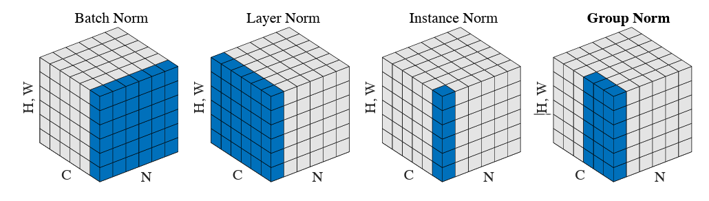
二、批量归一化（BN）

Batch Normalization（BN）是一种用于加速深度神经网络训练并提高其稳定性的技术，最初由Google 2015 年提出（论文：《Batch Normalization: Accelerating Deep Network Training by Reducing Internal Covariate Shift》）。BN 的核心思想是通过对每一层的输入进行归一化，减少内部协变量偏移（Internal Covariate Shift），从而使网络更容易训练。

2.1 操作流程

x 的形状：(batch_size, num_features, height, width)（B, C, H, W）

计算 mini-batch 的均值和方差，对当前 mini-batch 的输入\(x_i\)维度可以是向量、矩阵或张量），计算均值和方差，其中 m m m 是 mini-batch 的大小： \(\begin{array}{l} \mu_B=\frac{1}{m}\sum_{i=1}^m x_i\\ \sigma_B^2=\frac{1}{m}\sum_{i=1}^m (x_i-\mu_B)^2 \end{array}\)
标准化，将输入标准化为均值为 0、方差为 1 的分布，\(\epsilon\)是一个小的常数，用于防止除以零： \(\hat{x}_i=\frac{x_i-\mu_B}{\sqrt{\sigma_B^2+\epsilon}}\)
缩放和平移：引入可学习的参数 \(\gamma\)（缩放）和 \(\beta\)（平移），对标准化后的数据进行线性变换，以保持模型的表达能力： \(y_i=\gamma \hat{x}_i+\beta\)

2.2 优缺点

优点
1. 加速训练：通过减少内部协变量偏移，BN 使每一层的输入分布更稳定，从而加速梯度下降的收敛。允许使用更高的学习率，减少训练时间。
2. 提高稳定性：减少了梯度消失或爆炸的风险，使深层网络更容易训练。
3. 正则化效果：由于 mini-batch 的随机性，BN 引入了一些噪声，类似于 Dropout，具有一定的正则化效果，可能减少对过拟合的依赖。
4. 减少对参数初始化的敏感性：BN 使模型对权重初始化的选择不那么敏感，简化了超参数调整
缺点
1. 对小 batch size 敏感：当 mini-batch 较小时，均值和方差的估计不准确，导致 BN 性能下降。
2. 不适合某些任务：在动态网络（如循环神经网络 RNN）或某些生成模型中，BN 的效果可能不如预期，因为输入分布随时间变化较大。

2.3 代码实现

  
import torch

nn.BatchNorm2d(num_features)

class CustomBatchNorm2d(nn.Module):
    def __init__(self, num_features, eps=1e-5, momentum=0.1):
        super(CustomBatchNorm2d, self).__init__()
        self.num_features = num_features  # 通道数
        self.eps = eps  # 防止除以零的小值
        self.momentum = momentum  # 移动平均的动量

        # 可学习的参数：gamma（缩放）和 beta（平移）
        self.gamma = nn.Parameter(torch.ones(1, num_features, 1, 1))
        self.beta = nn.Parameter(torch.zeros(1, num_features, 1, 1))

        # 全局均值和方差，用于推理阶段
        self.register_buffer('running_mean', torch.zeros(1, num_features, 1, 1))
        self.register_buffer('running_var', torch.ones(1, num_features, 1, 1))
        self.register_buffer('num_batches_tracked', torch.tensor(0, dtype=torch.long))

    def forward(self, x):
        # x 的形状：(batch_size, num_features, height, width)
        if self.training:
            # 训练模式：计算 mini-batch 的均值和方差,沿 batch, height, width 轴
            batch_mean = x.mean(dim=(0, 2, 3), keepdim=True)
            batch_var = x.var(dim=(0, 2, 3), unbiased=False, keepdim=True)  

            # 更新全局均值和方差（使用移动平均）
            self.running_mean = (1 - self.momentum) * self.running_mean + self.momentum * batch_mean
            self.running_var = (1 - self.momentum) * self.running_var + self.momentum * batch_var
            self.num_batches_tracked += 1

            # 标准化
            x_hat = (x - batch_mean) / torch.sqrt(batch_var + self.eps)
        else:
            # 推理模式：使用全局均值和方差
            x_hat = (x - self.running_mean) / torch.sqrt(self.running_var + self.eps)

        # 缩放和平移
        out = self.gamma * x_hat + self.beta
        return out

三、层归一化（LN）

Layer Normalization（LN）是由 Jimmy Lei Ba 等人在 2016 年提出的一种归一化技术（论文：《Layer Normalization》）。Layer Normalization 对每个样本的特征（即沿 L（sequence_length）和 C（channels）维度）进行归一化，不依赖于 batch 维度。针对 [B, L, C] 输入，LN 对每个样本的 [L, C] 特征计算均值和方差，使其标准化为均值为 0、方差为 1 的分布，然后通过可学习的缩放和平移参数调整输出。这种方式特别适合序列模型（如 Transformer）或小批量场景。

3.1 操作流程

x 的形状：(batch_size, sequence_length, channels)（B, L, C）

计算单个样本的均值和方差，对每个样本（batch 维度的一个元素），沿 L（序列长度）和 C（通道）维度计算均值，方差： \(\begin{array}{l} \mu_i=\frac{1}{L\cdot C}\sum_{L\cdot C} x_{i,l,c}\\ \sigma_i^2=\frac{1}{L\cdot C}\sum_{i=1}^m (x_{i,l,c}-\mu_i)^2 \end{array}\)
标准化，将输入标准化为均值为 0、方差为 1 的分布，\(\epsilon\)是一个小的常数，用于防止除以零： \(\hat{x}_{i,l,c}=\frac{x_{i,l,c}-\mu_i}{\sqrt{\sigma_i^2+\epsilon}}\)
缩放和平移：引入可学习的参数 \(\gamma\)（缩放）和 \(\beta\)（平移），对标准化后的数据进行线性变换，以保持模型的表达能力： \(y_{i,l,c}=\gamma_{l,c} \hat{x}_{i,l,c}+\beta_{l,c}\)

3.2 优缺点

优点
1. 不依赖 batch 大小：LN 对每个样本独立计算均值和方差，适合小批量甚至单样本场景（batch_size=1）
2. 适合序列模型：对于 [B, L, C] 形状的输入（常见于 Transformer、RNN），LN 非常有效，因为它处理序列数据的动态变化能力强。
3. 正则化效果：由于 mini-batch 的随机性，BN 引入了一些噪声，类似于 Dropout，具有一定的正则化效果，可能减少对过拟合的依赖。
4. 减少对参数初始化的敏感性：BN 使模型对权重初始化的选择不那么敏感，简化了超参数调整
缺点
1. 任务特定性：对于某些卷积神经网络（CNN）任务，LN 可能不如 BN 有效，因为 BN 能利用 batch 维度的统计信息捕捉跨样本的模式。
2. 内存需求：LN 需要存储每个样本的均值和方差，以及与 [L, C] 形状匹配的 γ\gammaγ 和 β\betaβ 参数，内存开销可能较高。

3.3 代码实现

  
import torch

nn.LayerNorm(normalized_shape=x.shape[1:])

class CustomLayerNormSeq(nn.Module):
    def __init__(self, sequence_length, num_channels, eps=1e-5):
        super(CustomLayerNormSeq, self).__init__()
        self.sequence_length = sequence_length  # 序列长度 L
        self.num_channels = num_channels  # 通道数 C
        self.eps = eps  # 防止除以零的小值

        # 可学习的参数：gamma（缩放）和 beta（平移），形状为 [1, L, C]
        self.gamma = nn.Parameter(torch.ones(1, sequence_length, num_channels))
        self.beta = nn.Parameter(torch.zeros(1, sequence_length, num_channels))

    def forward(self, x):
        # x 的形状：(batch_size, sequence_length, num_channels)
        # 对每个样本的 (sequence_length, num_channels) 维度计算均值和方差,沿 sequence_length, num_channels 轴
        mean = x.mean(dim=(1, 2), keepdim=True) 
        var = x.var(dim=(1, 2), unbiased=False, keepdim=True)  

        # 标准化
        x_hat = (x - mean) / torch.sqrt(var + self.eps)

        # 缩放和平移
        out = self.gamma * x_hat + self.beta
        return out

四、分组归一化（GN）

Group Normalization（GN）是由 Yuxin Wu 和 Kaiming He 在 2018 年提出的一种归一化技术（论文：《Group Normalization》）。GN 是 BN 和 LN 的一种折中方案，旨在解决 BN 对小批量大小的敏感性，同时保留一定的跨样本统计信息。GN 将输入的通道（channels）分成若干组（groups），然后对每组内的特征进行归一化。针对 [B, L, C] 输入，GN 在每个样本的每组通道内计算均值和方差，适合小批量场景和序列数据处理。GN 的核心思想是将通道维度划分为组，沿组内的序列长度（L）和部分通道（C/G）计算统计量，从而在 BN 和 LN 之间取得平衡。

4.1 操作流程

x 的形状：(batch_size, num_features, height, width)（B, C, H, W）

通道分组：将通道维度 C 均分为 G 组，每组包含 C/G 个通道。输入张量重塑为 [B, G, C/G, H, W]，
计算每组的均值和方差，对每个样本的每组特征计算均值，方差，其中\(i\)是 batch 索引，\(g\)是组索引，\(c'\) 是组内通道索引：

\[\begin{array}{l} \mu_{i,g}=\frac{1}{(C/G)\cdot H\cdot W}\sum_{c',h,w} x_{i,g,c',h,w}\\ \sigma_{i,g}^2=\frac{1}{L\cdot C}\sum_{c',h,w} (x_{i,g,c',h,w}-\mu_{i,g})^2 \end{array}\]

标准化，将输入标准化为均值为 0、方差为 1 的分布，\(\epsilon\)是一个小的常数，用于防止除以零： \(\hat{x}_{i,g,c',h,w}=\frac{x_{i,g,c',h,w}-\mu_{i,g}}{\sqrt{\sigma_{i,g}^2+\epsilon}}\)
缩放和平移：引入可学习的参数 \(\gamma\)（缩放）和 \(\beta\)（平移），对标准化后的数据进行线性变换，以保持模型的表达能力： \(y_{i,g,c',h,w}=\gamma_{g,c',h,w} \hat{x}_{i,g,c',h,w}+\beta_{g,c',h,w}\)

4.2 优缺点

优点
1. 对小批量大小鲁棒：GN 在每组内计算统计量，不依赖整个 batch，适合小批量（如 batch_size=1）或单样本场景。
2. 介于 BN 和 LN 之间：GN 通过分组保留了部分跨通道的统计信息（相比 LN），同时避免了 BN 对 batch 大小的依赖。
3. 正则化效果：由于 mini-batch 的随机性，BN 引入了一些噪声，类似于 Dropout，具有一定的正则化效果，可能减少对过拟合的依赖。
4. 减少对参数初始化的敏感性：BN 使模型对权重初始化的选择不那么敏感，简化了超参数调整
缺点
1. 组数选择敏感：GN 的性能依赖于组数 G 的选择。组数过大（接近 LN）或过小（接近 BN）可能影响效果，需通过实验调整。
2. 对大批量场景的竞争力：在大批量场景中，BN 可能优于 GN，因为 BN 利用整个 batch 的统计信息提供更强的正则化。

4.3 代码实现

  
import torch

nn.GroupNorm(num_groups, num_channels)

class CustomGroupNorm2d(nn.Module):
    def __init__(self, num_channels, num_groups, eps=1e-5):
        super(CustomGroupNorm2d, self).__init__()
        self.num_channels = num_channels  # 通道数 C
        self.num_groups = num_groups  # 组数 G
        assert num_channels % num_groups == 0, "num_channels must be divisible by num_groups"
        self.eps = eps  # 防止除以零的小值

        # 可学习的参数：gamma（缩放）和 beta（平移），形状为 [1, num_channels, 1, 1]
        self.gamma = nn.Parameter(torch.ones(1, num_channels, 1, 1))
        self.beta = nn.Parameter(torch.zeros(1, num_channels, 1, 1))

    def forward(self, x):
        # x 的形状：(batch_size, num_channels, height, width)
        B, C, H, W = x.shape
        G = self.num_groups

        # 重塑输入为 (batch_size, num_groups, num_channels/num_groups, height, width)
        x = x.view(B, G, C // G, H, W)

        # 对每组 (num_channels/num_groups, height, width) 维度计算均值和方差,沿组内通道、高度和宽度轴计算均值
        mean = x.mean(dim=(2, 3, 4), keepdim=True)  
        var = x.var(dim=(2, 3, 4), unbiased=False, keepdim=True) 

        # 标准化
        x_hat = (x - mean) / torch.sqrt(var + self.eps)

        # 重塑回原始形状 (batch_size, num_channels, height, width)
        x_hat = x_hat.view(B, C, H, W)

        # 缩放和平移，gamma 和 beta 广播到 (batch_size, num_channels, height, width)
        out = self.gamma * x_hat + self.beta
        return out

五、单样本归一化（IN）

是针对单个样本进行标准化，在H，W上进行归一化，也就是与batch和layer都无关，执行完有B,C个均值，B,C个方差。每个样本实例的通道有自己的均值和方差。约等于B=1的BN，但是BN 在训练时会维护全局均值和方差（通过移动平均）

5.1 操作流程

x 的形状：(batch_size, num_features, height, width)（B, C, H, W）

计算 mini-batch 的均值和方差，对当前 mini-batch 的输入\(x_i\)维度可以是向量、矩阵或张量），计算均值和方差，其中 m m m 是 mini-batch 的大小： \(\begin{array}{l} \mu_{b,c}=\frac{1}{H\cdot W}\sum_{h,w} x_{b,c,h,w}\\ \sigma_{b,c}^2=\frac{1}{H\cdot W}\sum_{h,w} (x_{b,c,h,w}-\mu_{b,c})^2 \end{array}\)
标准化，将输入标准化为均值为 0、方差为 1 的分布，\(\epsilon\)是一个小的常数，用于防止除以零： \(\hat{x}_{b,c,h,w}=\frac{x_{b,c,h,w}-\mu_{b,c}}{\sqrt{\sigma_{b,c}^2+\epsilon}}\)
缩放和平移：引入可学习的参数 \(\gamma\)（缩放）和 \(\beta\)（平移），对标准化后的数据进行线性变换，以保持模型的表达能力： \(y_{b,c,h,w}=\gamma_c \hat{x}_{b,c,h,w}+\beta_c\)

5.2 优缺点

优点
1. 不依赖 batch 大小：IN 对每个样本和通道独立归一化，适合小批量甚至单样本场景（如 batch_size=1）。
2. 适合生成模型：IN 在风格迁移、GAN 等任务中表现优异，因为它规范化每个样本的特征，保留图像的对比度等特性，避免 batch 统计量对样本特异性的干扰。
3. 计算简单：IN 的计算仅涉及每个样本的每个通道，逻辑简单，易于实现。
缺点
1. 任务局限性：IN 主要用于生成模型，在常规分类任务（如 ResNet 上的图像分类）中效果通常不如 BN 或 GN。

5.3 代码实现

  
nn.InstanceNorm2d(num_features)

class CustomInstanceNorm2d(nn.Module):
    def __init__(self, num_channels, eps=1e-5):
        super(CustomInstanceNorm2d, self).__init__()
        self.num_channels = num_channels  # 通道数 C
        self.eps = eps  # 防止除以零的小值

        # 可学习的参数：gamma（缩放）和 beta（平移），形状为 [1, num_channels, 1, 1]
        self.gamma = nn.Parameter(torch.ones(1, num_channels, 1, 1))
        self.beta = nn.Parameter(torch.zeros(1, num_channels, 1, 1))

    def forward(self, x):
        # x 的形状：(batch_size, num_channels, height, width)
        B, C, H, W = x.shape

        # 对每个样本的每个通道 (height, width) 维度计算均值和方差
        mean = x.mean(dim=(2, 3), keepdim=True)  # 沿 height 和 width 轴计算均值
        var = x.var(dim=(2, 3), unbiased=False, keepdim=True)  # 沿 height 和 width 轴计算方差

        # 标准化
        x_hat = (x - mean) / torch.sqrt(var + self.eps)

        # 缩放和平移，gamma 和 beta 广播到 (batch_size, num_channels, height, width)
        out = self.gamma * x_hat + self.beta
        return out

1. Internal Covariate Shift

Training deep neural networks is complicated because changes in the parameters of earlier layers cause the distribution of each layer’s input to change during training. This in turn forces the model to use a lower learning rate and a very careful parameter initialization strategy, which slows down training; models with saturating nonlinearities also become very hard to train.

This phenomenon, in which the distribution of a layer’s input data changes, is called internal covariate shift, and BN was proposed to solve it.

2.1 How to Understand Internal Covariate Shift

During the training of a deep neural network, the process in which changes of the network parameters cause the data distribution of the intermediate layers to change is called Internal Covariate Shift in the original paper.

So why does the data distribution of the intermediate layers change?

In a deep neural network we can view each layer as applying a transformation to the input signal (ignoring activations for the moment, since activation functions do not change the distribution of the input data):

\[Z = W \cdot X + B\]

where \(W\) and \(B\) are the parameters learned by the model; this formula covers both fully connected layers and convolution layers.

As SGD updates the parameters, and as each layer’s input data passes through the formula, the distribution of \(Z\) keeps changing. Every layer therefore has to keep adapting to a new distribution, and this process is what we call Internal Covariate Shift. The difficulty of training deep networks is that each layer’s input is affected by the parameters of all preceding layers — so as the network gets deeper, tiny changes in the parameters get amplified.

2.2 Problems Caused by Internal Covariate Shift

Layers have to keep adapting to a new distribution, which slows down learning.
Layer inputs easily fall into a nonlinear saturation region, which slows down convergence; this effect is amplified as the network gets deeper.
As the network deepens, the input \(x\) to later layers grows larger. If a Sigmoid-type activation is used, each layer’s input can easily move into the nonlinear saturation region, where gradients become very small or even close to \(0\). Parameter updates then slow down, which in turn slows down convergence.

Saturation and the resulting vanishing gradients are usually addressed by using rectified linear activations (\(ReLU(x)=max(x,0)\)), better parameter initialization, and a small learning rate. However, if we could keep the distribution of the nonlinear inputs more stable during training, the optimizer would be much less likely to fall into saturation and training would speed up.

2.3 Some Attempts at Reducing Internal Covariate Shift

Whitening: linearly transform the inputs to have zero mean and unit variance, and decorrelate them. Because whitening changes the distribution of every layer, it changes the representational capacity of the data in that layer. Information learned by the lower layers is lost by the whitening operation, and whitening is also computationally expensive.
Normalization
Although normalization alleviates the ICS problem and makes the input distribution of each layer stable, it also causes a loss of representational capacity.

2.4 Common Normalization Layers

2. Batch Normalization (BN)

Batch Normalization (BN) is a technique for accelerating the training of deep neural networks and improving their stability, first proposed by Google in 2015 (paper: Batch Normalization: Accelerating Deep Network Training by Reducing Internal Covariate Shift). The core idea of BN is to normalize the input of each layer to reduce internal covariate shift, which makes the network easier to train.

2.1 Procedure

The shape of x: (batch_size, num_features, height, width), i.e. (B, C, H, W).

Compute the mean and variance of the mini-batch. For the current mini-batch, the input \(x_i\) may have dimensions of a vector, a matrix, or a tensor; compute the mean and variance, where \(m\) is the size of the mini-batch: \(\begin{array}{l} \mu_B=\frac{1}{m}\sum_{i=1}^m x_i\\ \sigma_B^2=\frac{1}{m}\sum_{i=1}^m (x_i-\mu_B)^2 \end{array}\)
Normalize: standardize the inputs into a distribution with mean 0 and variance 1, where \(\epsilon\) is a small constant that prevents division by zero: \(\hat{x}_i=\frac{x_i-\mu_B}{\sqrt{\sigma_B^2+\epsilon}}\)
Scale and shift: introduce the learnable parameters \(\gamma\) (scale) and \(\beta\) (shift) and apply a linear transformation to the normalized data so that the model keeps its representational capacity: \(y_i=\gamma \hat{x}_i+\beta\)

2.2 Pros and Cons

Pros
1. Faster training: by reducing internal covariate shift, BN makes the input distribution of each layer more stable, which accelerates gradient descent. It allows a higher learning rate and reduces training time.
2. Improved stability: it reduces the risk of vanishing or exploding gradients, making deep networks easier to train.
3. Regularization effect: because of the randomness of the mini-batch, BN introduces some noise similar to Dropout, giving it a mild regularization effect that may reduce reliance on other anti-overfitting measures.
4. Less sensitivity to parameter initialization: BN makes the model less sensitive to the choice of weight initialization and simplifies hyper-parameter tuning.
Cons
1. Sensitive to small batch sizes: with a small mini-batch the estimates of mean and variance are inaccurate, which degrades BN’s performance.
2. Not suited to certain tasks: in dynamic networks (such as recurrent neural networks, RNNs) or some generative models, BN may not perform as expected because the input distribution varies considerably over time.

2.3 Code Implementation

  
import torch

nn.BatchNorm2d(num_features)

class CustomBatchNorm2d(nn.Module):
    def __init__(self, num_features, eps=1e-5, momentum=0.1):
        super(CustomBatchNorm2d, self).__init__()
        self.num_features = num_features  # number of channels
        self.eps = eps  # small value preventing division by zero
        self.momentum = momentum  # momentum of the moving average

        # Learnable parameters: gamma (scale) and beta (shift)
        self.gamma = nn.Parameter(torch.ones(1, num_features, 1, 1))
        self.beta = nn.Parameter(torch.zeros(1, num_features, 1, 1))

        # Global mean and variance, used at inference time
        self.register_buffer('running_mean', torch.zeros(1, num_features, 1, 1))
        self.register_buffer('running_var', torch.ones(1, num_features, 1, 1))
        self.register_buffer('num_batches_tracked', torch.tensor(0, dtype=torch.long))

    def forward(self, x):
        # shape of x: (batch_size, num_features, height, width)
        if self.training:
            # Training mode: compute the mini-batch mean and variance
            # along the batch, height and width axes
            batch_mean = x.mean(dim=(0, 2, 3), keepdim=True)
            batch_var = x.var(dim=(0, 2, 3), unbiased=False, keepdim=True)  

            # Update the global mean and variance (moving average)
            self.running_mean = (1 - self.momentum) * self.running_mean + self.momentum * batch_mean
            self.running_var = (1 - self.momentum) * self.running_var + self.momentum * batch_var
            self.num_batches_tracked += 1

            # Normalize
            x_hat = (x - batch_mean) / torch.sqrt(batch_var + self.eps)
        else:
            # Inference mode: use the global mean and variance
            x_hat = (x - self.running_mean) / torch.sqrt(self.running_var + self.eps)

        # Scale and shift
        out = self.gamma * x_hat + self.beta
        return out

3. Layer Normalization (LN)

Layer Normalization (LN) is a normalization technique proposed by Jimmy Lei Ba et al. in 2016 (paper: Layer Normalization). Layer Normalization normalizes the features of each individual sample (that is, along the L (sequence_length) and C (channels) dimensions) and does not depend on the batch dimension. For an input of shape [B, L, C], LN computes the mean and variance over the [L, C] features of each sample, standardizing them into a distribution with mean 0 and variance 1, and then adjusts the output with learnable scale and shift parameters. This makes it particularly suitable for sequence models (such as Transformers) or small-batch scenarios.

3.1 Procedure

The shape of x: (batch_size, sequence_length, channels), i.e. (B, L, C).

Compute the mean and variance of a single sample. For each sample (one element of the batch dimension), compute the mean and variance along the L (sequence length) and C (channel) dimensions: \(\begin{array}{l} \mu_i=\frac{1}{L\cdot C}\sum_{L\cdot C} x_{i,l,c}\\ \sigma_i^2=\frac{1}{L\cdot C}\sum_{i=1}^m (x_{i,l,c}-\mu_i)^2 \end{array}\)
Normalize: standardize the inputs into a distribution with mean 0 and variance 1, where \(\epsilon\) is a small constant that prevents division by zero: \(\hat{x}_{i,l,c}=\frac{x_{i,l,c}-\mu_i}{\sqrt{\sigma_i^2+\epsilon}}\)
Scale and shift: introduce the learnable parameters \(\gamma\) (scale) and \(\beta\) (shift) and apply a linear transformation to the normalized data so that the model keeps its representational capacity: \(y_{i,l,c}=\gamma_{l,c} \hat{x}_{i,l,c}+\beta_{l,c}\)

3.2 Pros and Cons

Pros
1. Independent of batch size: LN computes the mean and variance for each sample independently, which suits small batches or even a single sample (batch_size=1).
2. Suited to sequence models: for inputs of shape [B, L, C] (common in Transformers and RNNs), LN is very effective because it handles the dynamic variation of sequence data well.
3. Regularization effect: because of the randomness of the mini-batch, BN introduces some noise similar to Dropout, giving it a mild regularization effect that may reduce reliance on other anti-overfitting measures.
4. Less sensitivity to parameter initialization: BN makes the model less sensitive to the choice of weight initialization and simplifies hyper-parameter tuning.
Cons
1. Task specificity: for certain convolutional neural network (CNN) tasks, LN may be less effective than BN, because BN can exploit the statistics of the batch dimension to capture cross-sample patterns.
2. Memory requirements: LN needs to store the mean and variance of each sample as well as the γ and β parameters matching the [L, C] shape, so the memory overhead may be relatively high.

3.3 Code Implementation

  
import torch

nn.LayerNorm(normalized_shape=x.shape[1:])

class CustomLayerNormSeq(nn.Module):
    def __init__(self, sequence_length, num_channels, eps=1e-5):
        super(CustomLayerNormSeq, self).__init__()
        self.sequence_length = sequence_length  # sequence length L
        self.num_channels = num_channels  # number of channels C
        self.eps = eps  # small value preventing division by zero

        # Learnable parameters: gamma (scale) and beta (shift), shape [1, L, C]
        self.gamma = nn.Parameter(torch.ones(1, sequence_length, num_channels))
        self.beta = nn.Parameter(torch.zeros(1, sequence_length, num_channels))

    def forward(self, x):
        # shape of x: (batch_size, sequence_length, num_channels)
        # Compute the mean and variance over the (sequence_length, num_channels)
        # dimensions of each sample, along the sequence_length and num_channels axes
        mean = x.mean(dim=(1, 2), keepdim=True) 
        var = x.var(dim=(1, 2), unbiased=False, keepdim=True)  

        # Normalize
        x_hat = (x - mean) / torch.sqrt(var + self.eps)

        # Scale and shift
        out = self.gamma * x_hat + self.beta
        return out

4. Group Normalization (GN)

Group Normalization (GN) is a normalization technique proposed by Yuxin Wu and Kaiming He in 2018 (paper: Group Normalization). GN is a compromise between BN and LN: it aims to solve BN’s sensitivity to small batch sizes while retaining some cross-sample statistical information. GN divides the input channels into several groups and then normalizes the features within each group. For an input of shape [B, L, C], GN computes the mean and variance within each group of channels for each sample, which suits small-batch scenarios and sequence data. The core idea of GN is to partition the channel dimension into groups and compute statistics along the sequence length (L) and the channels within the group (C/G), thus striking a balance between BN and LN.

4.1 Procedure

The shape of x: (batch_size, num_features, height, width), i.e. (B, C, H, W).

Group the channels: split the channel dimension C evenly into G groups, each containing C/G channels. The input tensor is reshaped into [B, G, C/G, H, W].
Compute the mean and variance of each group. For each sample and each group of features, compute the mean and variance, where \(i\) is the batch index, \(g\) the group index, and \(c'\) the channel index within the group:

\[\begin{array}{l} \mu_{i,g}=\frac{1}{(C/G)\cdot H\cdot W}\sum_{c',h,w} x_{i,g,c',h,w}\\ \sigma_{i,g}^2=\frac{1}{L\cdot C}\sum_{c',h,w} (x_{i,g,c',h,w}-\mu_{i,g})^2 \end{array}\]

Normalize: standardize the inputs into a distribution with mean 0 and variance 1, where \(\epsilon\) is a small constant that prevents division by zero: \(\hat{x}_{i,g,c',h,w}=\frac{x_{i,g,c',h,w}-\mu_{i,g}}{\sqrt{\sigma_{i,g}^2+\epsilon}}\)
Scale and shift: introduce the learnable parameters \(\gamma\) (scale) and \(\beta\) (shift) and apply a linear transformation to the normalized data so that the model keeps its representational capacity: \(y_{i,g,c',h,w}=\gamma_{g,c',h,w} \hat{x}_{i,g,c',h,w}+\beta_{g,c',h,w}\)

4.2 Pros and Cons

Pros
1. Robust to small batch sizes: GN computes statistics within each group and does not depend on the whole batch, so it suits small batches (such as batch_size=1) or single-sample scenarios.
2. Between BN and LN: through grouping, GN retains part of the cross-channel statistical information (compared with LN) while avoiding BN’s dependence on batch size.
3. Regularization effect: because of the randomness of the mini-batch, BN introduces some noise similar to Dropout, giving it a mild regularization effect that may reduce reliance on other anti-overfitting measures.
4. Less sensitivity to parameter initialization: BN makes the model less sensitive to the choice of weight initialization and simplifies hyper-parameter tuning.
Cons
1. Sensitive to the choice of the number of groups: GN’s performance depends on the choice of the number of groups G. Too many groups (approaching LN) or too few (approaching BN) may hurt the result, so it must be tuned experimentally.
2. Less competitive in large-batch scenarios: with large batches BN may outperform GN, because BN exploits the statistics of the whole batch and provides stronger regularization.

4.3 Code Implementation

  
import torch

nn.GroupNorm(num_groups, num_channels)

class CustomGroupNorm2d(nn.Module):
    def __init__(self, num_channels, num_groups, eps=1e-5):
        super(CustomGroupNorm2d, self).__init__()
        self.num_channels = num_channels  # number of channels C
        self.num_groups = num_groups  # number of groups G
        assert num_channels % num_groups == 0, "num_channels must be divisible by num_groups"
        self.eps = eps  # small value preventing division by zero

        # Learnable parameters: gamma (scale) and beta (shift), shape [1, num_channels, 1, 1]
        self.gamma = nn.Parameter(torch.ones(1, num_channels, 1, 1))
        self.beta = nn.Parameter(torch.zeros(1, num_channels, 1, 1))

    def forward(self, x):
        # shape of x: (batch_size, num_channels, height, width)
        B, C, H, W = x.shape
        G = self.num_groups

        # Reshape the input to (batch_size, num_groups, num_channels/num_groups, height, width)
        x = x.view(B, G, C // G, H, W)

        # Compute the mean and variance of each group over the
        # (num_channels/num_groups, height, width) dimensions,
        # along the within-group channel, height and width axes
        mean = x.mean(dim=(2, 3, 4), keepdim=True)  
        var = x.var(dim=(2, 3, 4), unbiased=False, keepdim=True) 

        # Normalize
        x_hat = (x - mean) / torch.sqrt(var + self.eps)

        # Reshape back to the original shape (batch_size, num_channels, height, width)
        x_hat = x_hat.view(B, C, H, W)

        # Scale and shift; gamma and beta are broadcast to
        # (batch_size, num_channels, height, width)
        out = self.gamma * x_hat + self.beta
        return out

5. Instance Normalization (IN)

Instance Normalization standardizes each individual sample, normalizing over H and W; it therefore depends on neither the batch nor the layer, and produces B×C means and B×C variances. The channels of each sample instance have their own mean and variance. It is roughly BN with B=1, except that BN maintains global mean and variance during training (through a moving average).

5.1 Procedure

The shape of x: (batch_size, num_features, height, width), i.e. (B, C, H, W).

Compute the mean and variance of the mini-batch. For the current mini-batch, the input \(x_i\) may have dimensions of a vector, a matrix, or a tensor; compute the mean and variance, where \(m\) is the size of the mini-batch: \(\begin{array}{l} \mu_{b,c}=\frac{1}{H\cdot W}\sum_{h,w} x_{b,c,h,w}\\ \sigma_{b,c}^2=\frac{1}{H\cdot W}\sum_{h,w} (x_{b,c,h,w}-\mu_{b,c})^2 \end{array}\)
Normalize: standardize the inputs into a distribution with mean 0 and variance 1, where \(\epsilon\) is a small constant that prevents division by zero: \(\hat{x}_{b,c,h,w}=\frac{x_{b,c,h,w}-\mu_{b,c}}{\sqrt{\sigma_{b,c}^2+\epsilon}}\)
Scale and shift: introduce the learnable parameters \(\gamma\) (scale) and \(\beta\) (shift) and apply a linear transformation to the normalized data so that the model keeps its representational capacity: \(y_{b,c,h,w}=\gamma_c \hat{x}_{b,c,h,w}+\beta_c\)

5.2 Pros and Cons

Pros
1. Independent of batch size: IN normalizes each sample and channel independently, which suits small batches or even a single sample (such as batch_size=1).
2. Suited to generative models: IN performs well in style transfer, GANs and similar tasks, because it normalizes the features of each sample, preserves properties such as image contrast, and avoids interference from batch statistics on sample-specific characteristics.
3. Simple computation: IN only involves each channel of each sample, so the logic is simple and easy to implement.
Cons
1. Limited applicability: IN is mainly used in generative models; on ordinary classification tasks (such as image classification with ResNet) it is usually less effective than BN or GN.

5.3 Code Implementation

  
nn.InstanceNorm2d(num_features)

class CustomInstanceNorm2d(nn.Module):
    def __init__(self, num_channels, eps=1e-5):
        super(CustomInstanceNorm2d, self).__init__()
        self.num_channels = num_channels  # number of channels C
        self.eps = eps  # small value preventing division by zero

        # Learnable parameters: gamma (scale) and beta (shift), shape [1, num_channels, 1, 1]
        self.gamma = nn.Parameter(torch.ones(1, num_channels, 1, 1))
        self.beta = nn.Parameter(torch.zeros(1, num_channels, 1, 1))

    def forward(self, x):
        # shape of x: (batch_size, num_channels, height, width)
        B, C, H, W = x.shape

        # Compute the mean and variance over the (height, width) dimensions
        # of each channel of each sample
        mean = x.mean(dim=(2, 3), keepdim=True)  # mean along the height and width axes
        var = x.var(dim=(2, 3), unbiased=False, keepdim=True)  # variance along the height and width axes

        # Normalize
        x_hat = (x - mean) / torch.sqrt(var + self.eps)

        # Scale and shift; gamma and beta are broadcast to
        # (batch_size, num_channels, height, width)
        out = self.gamma * x_hat + self.beta
        return out

Deep Learning (CV) , Basics