深度学习——模型

一、MLP

(1)Linear（线性层）

定义： Linear层是PyTorch等深度学习框架中的一个基本层类型，执行线性变换，即输出是输入向量与权重矩阵的乘积再加上偏置。

特点：

• 仅执行线性变换，不包含非线性激活函数。
• 是构建FC层或MLP的一部分，因为FC层或MLP通常在Linear层后面加上非线性激活函数。

(2)激活函数

https://zhuanlan.zhihu.com/p/690848035

(3)MLP（Multi-Layer Perceptron）

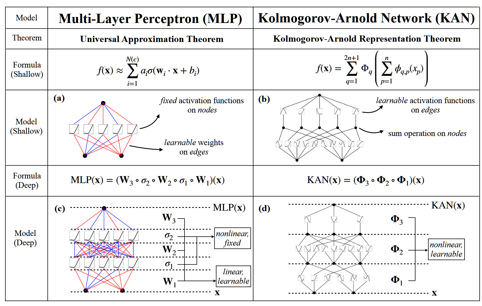
定义： MLP是多层感知机的缩写，是一种前馈神经网络，通常包括一个输入层、一个或多个隐藏层和一个输出层。每层中的神经元都与下一层的神经元完全连接。是由多个Linear和激活函数组成的

特点：

• MLP 是一种更高级别的神经网络结构，它包含多个层（输入层、隐藏层、输出层）。
• 各层之间是全连接的（即每个神经元都连接到下一层的每个神经元）。
• 使用非线性激活函数（如ReLU、Sigmoid、Tanh）以增加网络的表达能力。

(4)KAN

二、CNN

0、卷积神经网络基础

卷积

(1)标准卷积

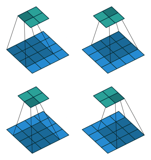
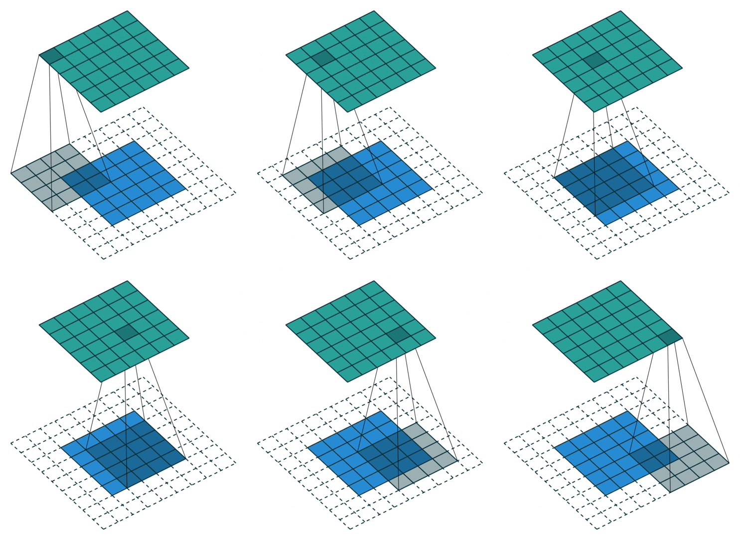
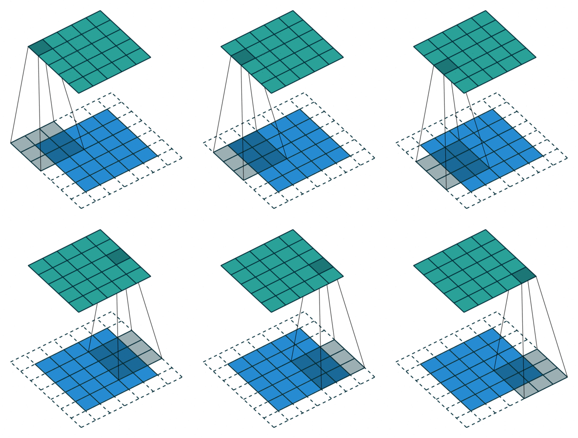
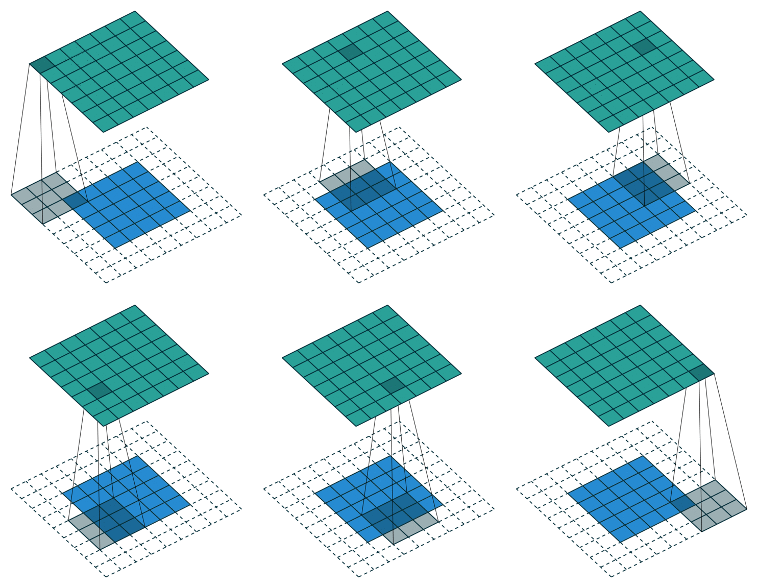
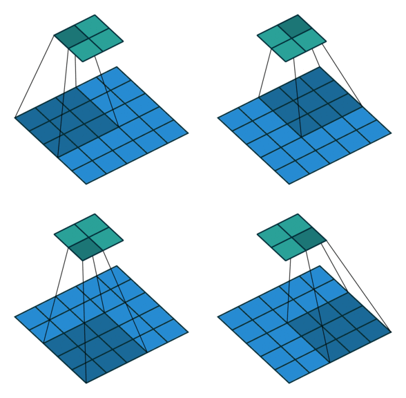
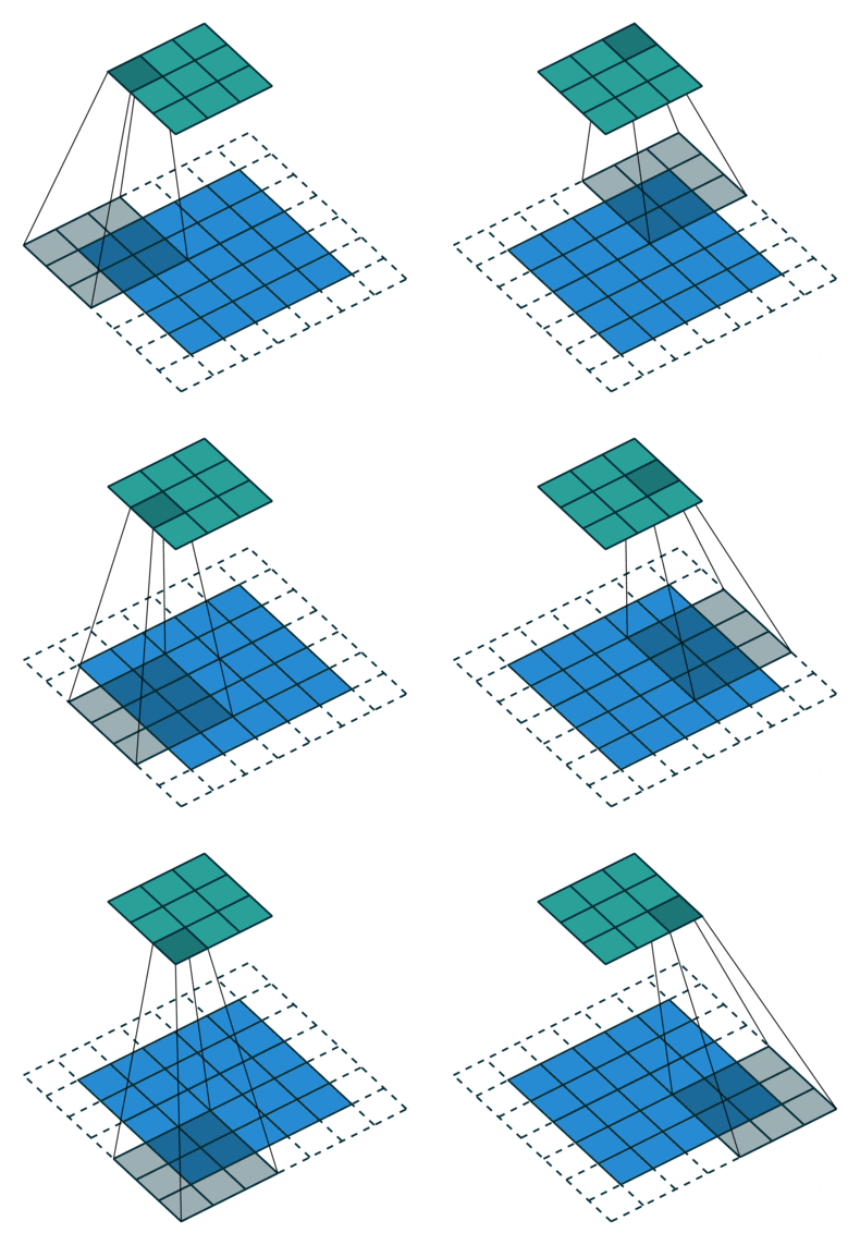
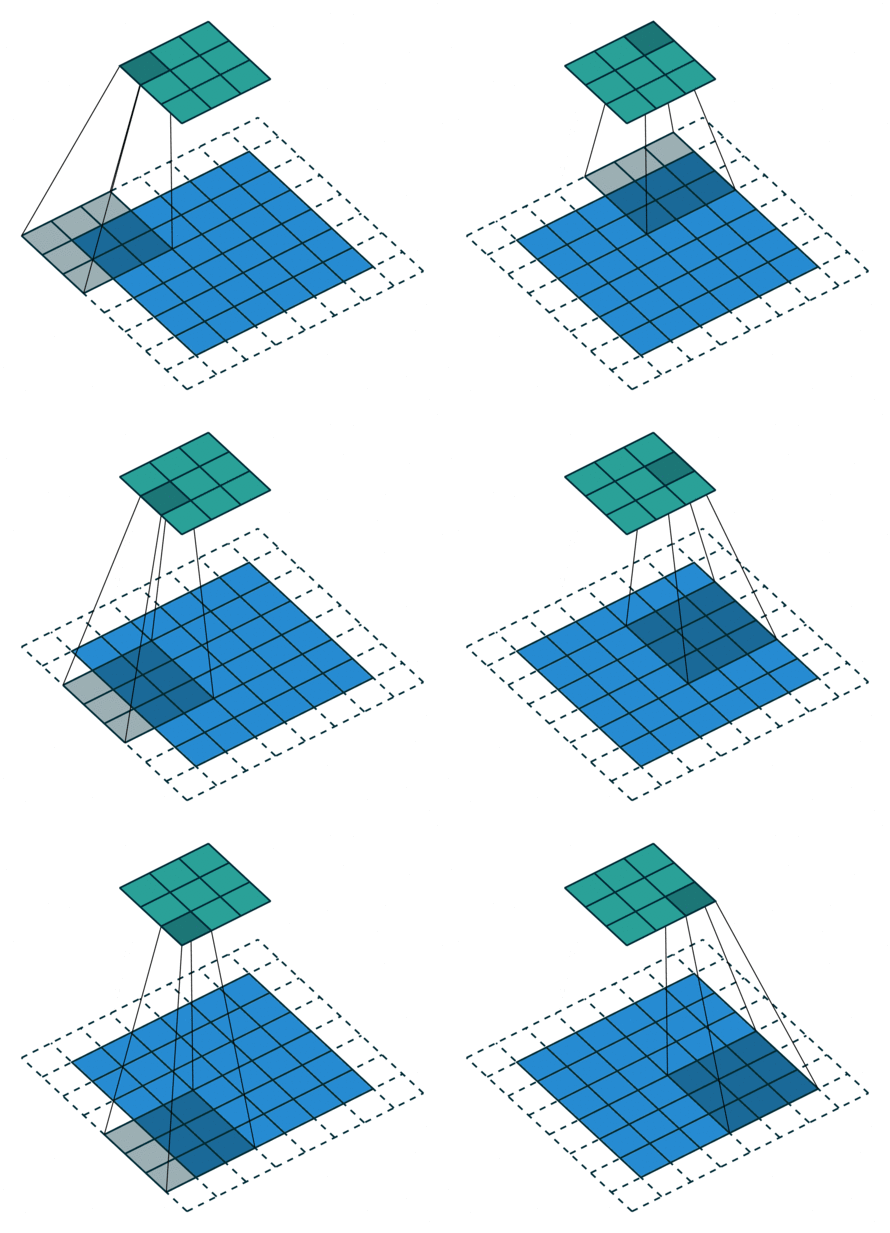
• Kernel size（核的大小）：卷积核的大小

• Stride（步长）：它定义了在图像中滑动时，Kernels的步长。

• Padding（填充）：Padding定义了图像边框的处理方式，卷积通过在输入边界周围填充来保持输出的大小等于输入图像的大小。

\[O=\frac{(I-Kernel\_size+2*Padding)}{Stride}+1\]

No padding, no strides

Arbitrary padding, no strides

Half padding, no strides

Full padding, no strides

No padding, strides

Padding, strides

Padding, strides (odd)

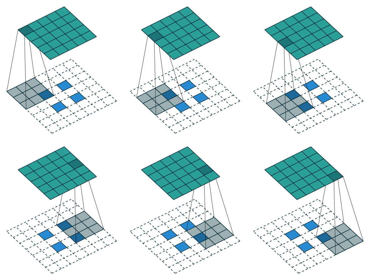
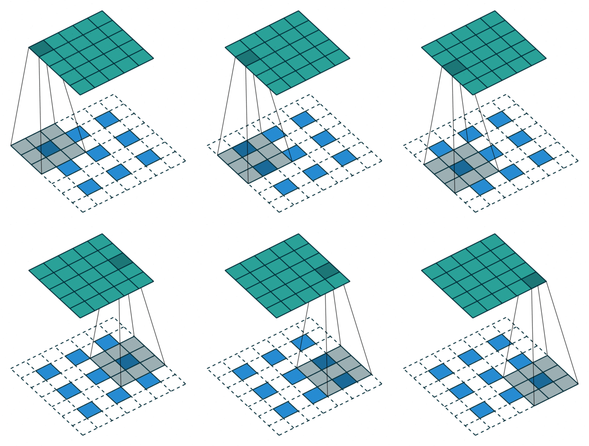
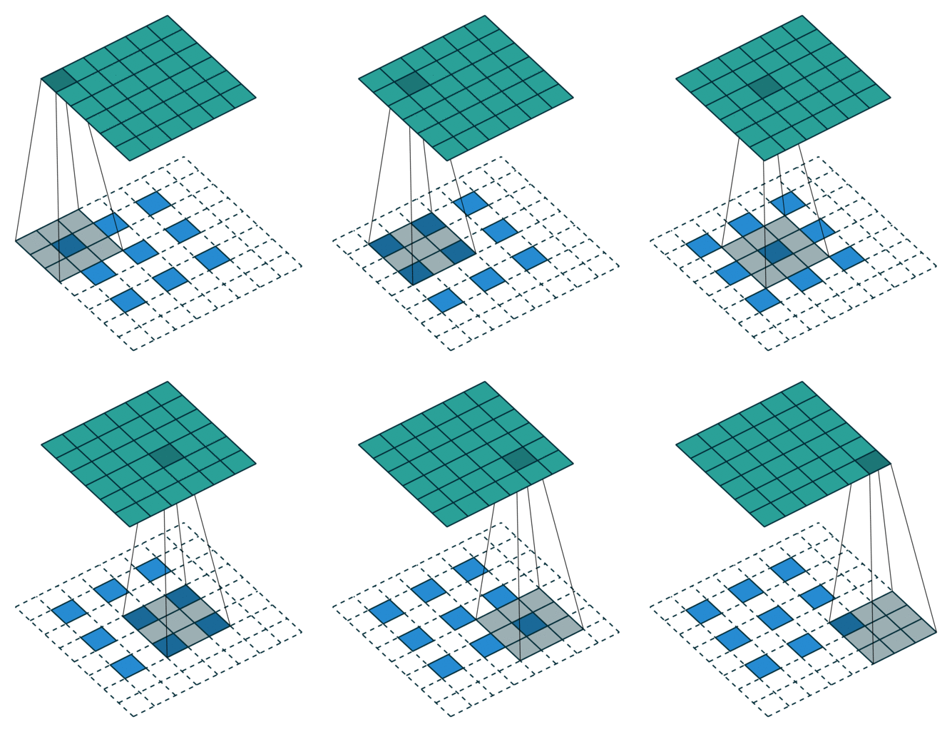
(2)转置卷积(反卷积)

No padding, no strides, transposed

Arbitrary padding, no strides, transposed

Half padding, no strides, transposed

Full padding, no strides, transposed

No padding, strides, transposed

Padding, strides, transposed

Padding, strides, transposed (odd)

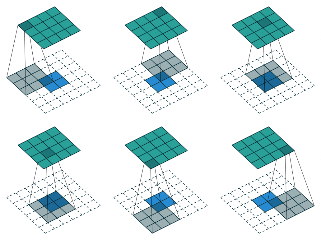
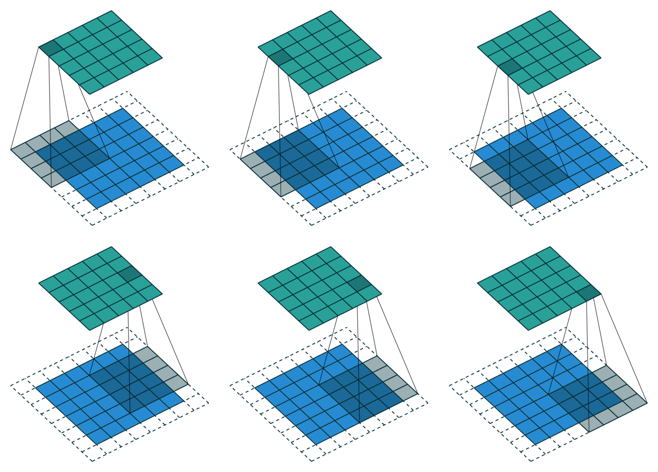
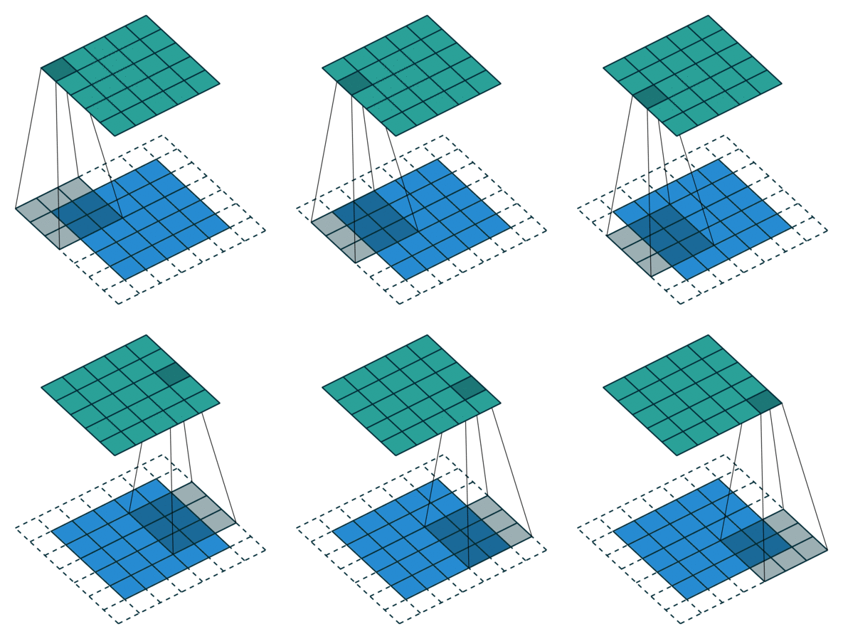
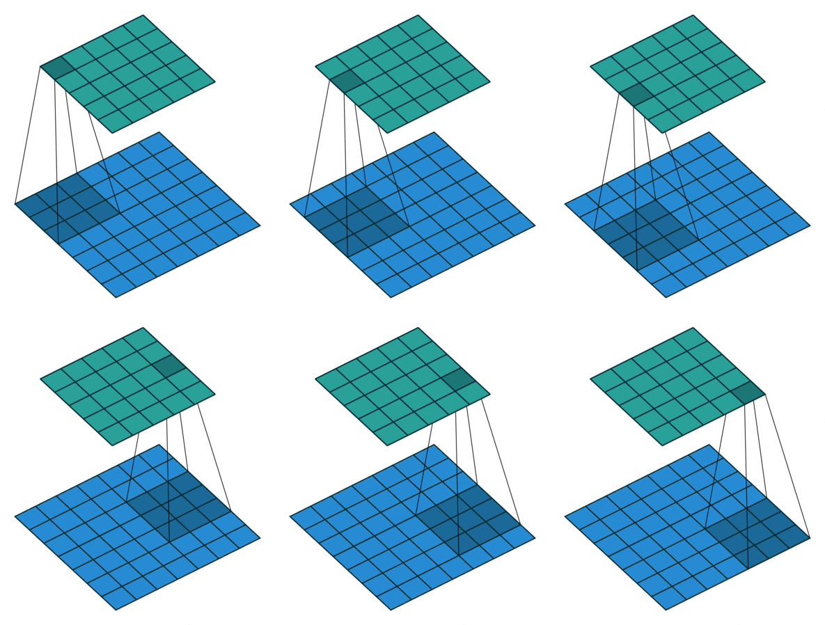
(3)空洞卷积

No padding, no stride, dilation

下采样(池化)

(1)最大池化、平均池化

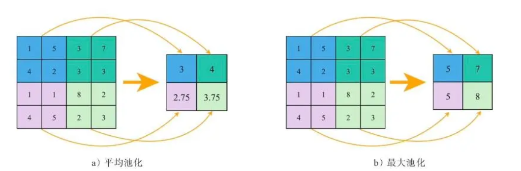
(2)卷积下采样

通过调整Kernel size（核的大小）、Stride（步长）、Padding（填充）实现下采样

(3)插值下采样

使用插值方法实现下采样

上采样

(1)反池化

反平均池化 首先还原成原来的大小，然后将池化结果中的每个值都填入其对应原始数据区域中相应位置即可（平均代替所有）

反最大池化 要求在池化过程中记录最大激活值的坐标位置，然后在反池化时，只把池化过程中最大激活值所在位置坐标值激活，其他的值设置为0.当然，这个过程只是一种近似。因为在池化过程中，除了最大值的位置，其他的值也是不为0的。

(2)反卷积

通过调整Kernel size（核的大小）、Stride（步长）、Padding（填充）等实现上采样

(3)子像素卷积

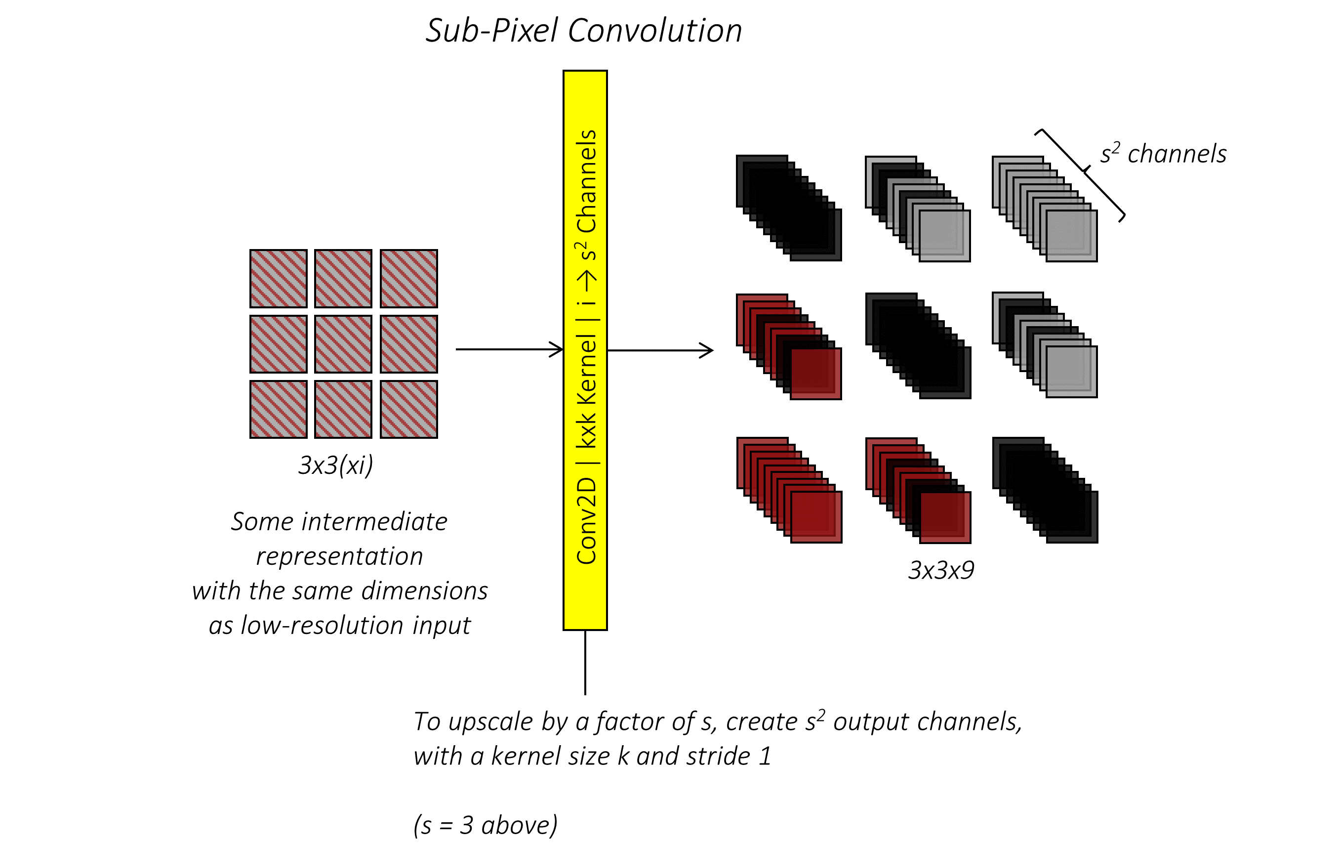
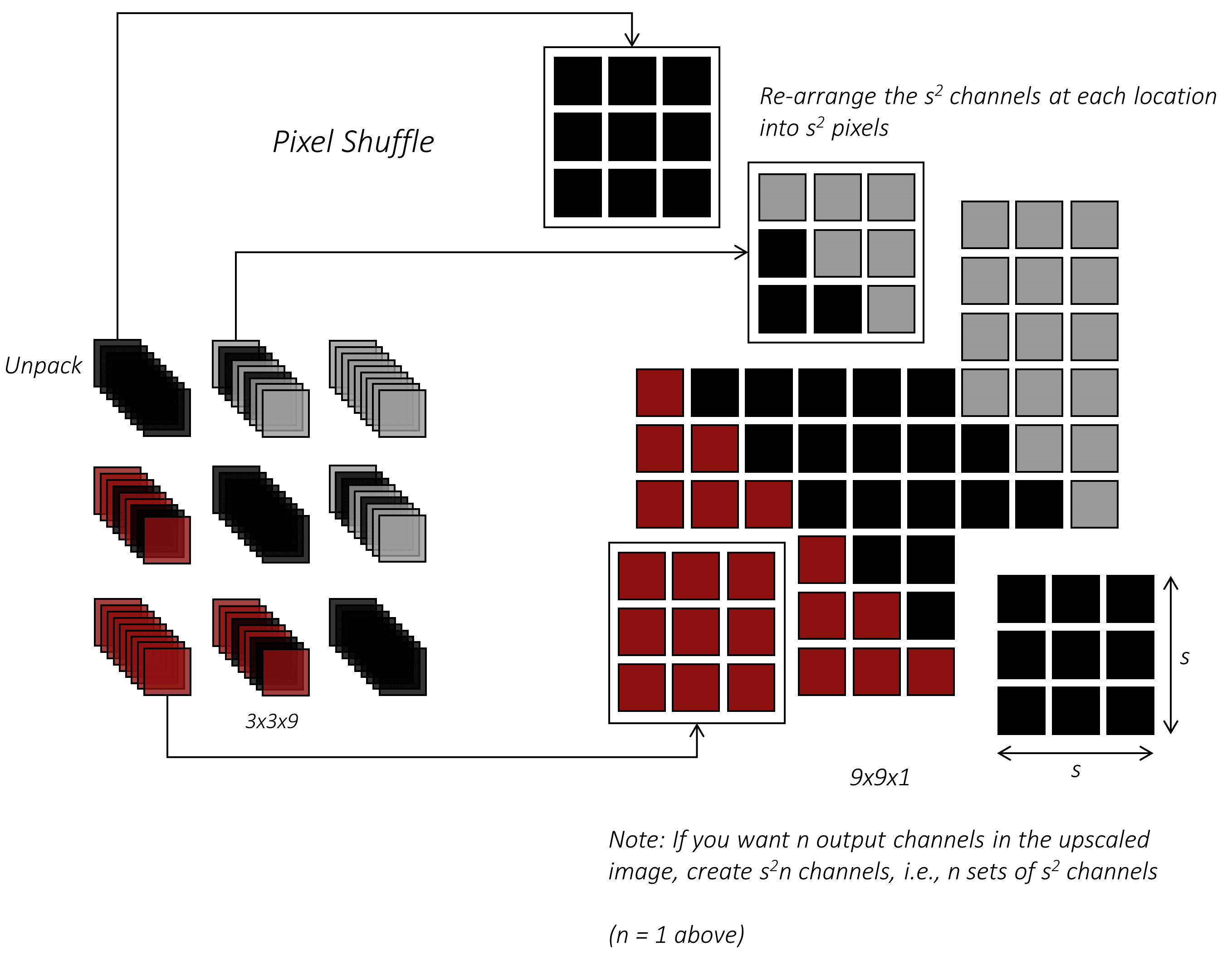
(4)插值

nearest、linear、bilinear、bicubic、trilinear、area等

1、AlexNet

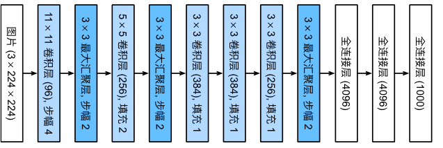
在AlexNet的第一层，卷积窗口的形状是 11×11。由于ImageNet中大多数图像的宽和高比MNIST图像的多10倍 以上，因此，需要一个更大的卷积窗口来捕获目标。第二层中的卷积窗口形状被缩减为 5×5，然后是 3×3。此 外，在第一层、第二层和第五层卷积层之后，加入窗口形状为 3×3、步幅为2的最大汇聚层。

AlexNet将sigmoid激活函数改为更简单的ReLU激活函数。一方面，ReLU激活函数的计算更简单，它 不需要如sigmoid激活函数那般复杂的求幂运算。另一方面，当使用不同的参数初始化方法时，ReLU激活函 数使训练模型更加容易。当sigmoid激活函数的输出非常接近于0或1时，这些区域的梯度几乎为0，因此反向 传播无法继续更新一些模型参数。相反，ReLU激活函数在正区间的梯度总是1。因此，如果模型参数没有正 确初始化，sigmoid函数可能在正区间内得到几乎为0的梯度，从而使模型无法得到有效的训练。

2、VGG

经典卷积神经网络的基本组成部分是下面的这个序列：

1. 带填充以保持分辨率的卷积层；
2. 非线性激活函数，如ReLU；
3. 池化层，如最大池化

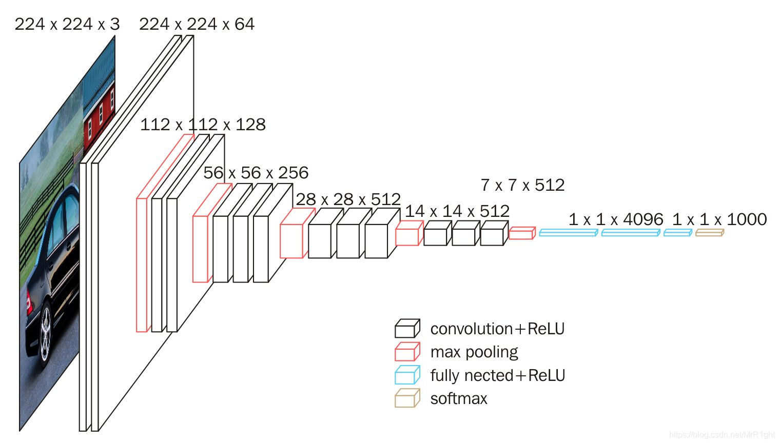
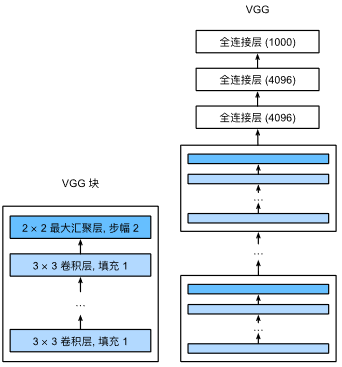
使用块的想法首先出现在牛津大学的视觉几何组的VGG网络中。通过使用循环和子程序，可以很容易地在任何现代深度学习框架的代码中实现这些重复的架构。

3、ResNet

（1）残差的思路

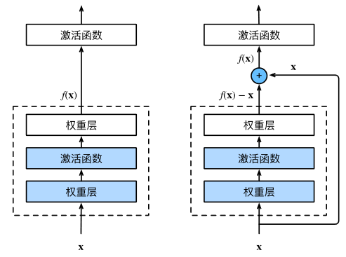
假设我们的原始输入为x，而希望学出的理想映射为f (x)。左图虚线框中的部分需要直接拟合出该映射f (x)，而右图虚线框中的部分则需要拟合出残差映射f (x)-x。残差映射在现实中往往更容易优化。恒等映射作为我们希望学出的理想映射f (x)，我们只需将右图虚线框内上方的加权运算（如仿射）的权重和偏置参数设成0，那么f (x)即为恒等映射。实际中，当理想映射f (x)极接近于恒等映射时，残差映射也易于捕捉恒等映射的细微波动。

（2）残差块

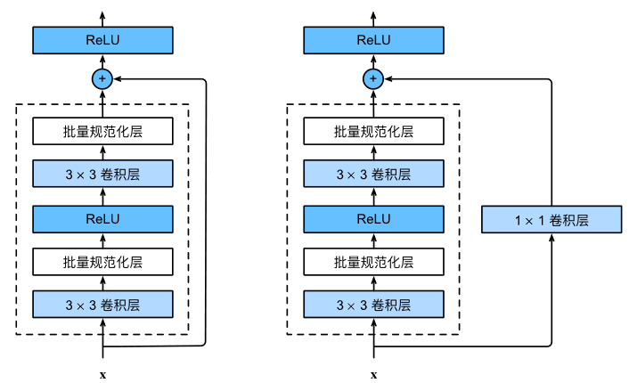
\(1\times1\)卷积的作用是调整通道

4、GoogLeNet（并行）

在GoogLeNet中，基本的卷积块被称为Inception块

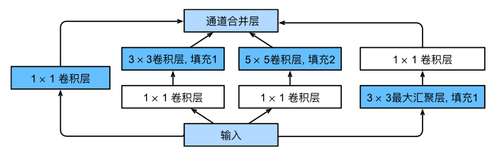
Inception块由四条并行路径组成。前三条路径使用窗口大小为 1×1、3×3 和 5×5 的卷积层，从不同空间大小中提取信息。中间的两条路径在输入上执行 1×1 卷积，以减少通道数，从而降低模型的复杂性。第四条路径使用 3×3 最大汇聚层，然后使用 1×1 卷积层来改变通道数。这四条路径都使用合适的填充来使输入与输出的高和宽一致，最后我们将每条线路的输出在通道维度上连结，并构成Inception块的输出在Inception块中，通常调整的超参数是每层输出通道数。

5、UNet

三、RNN

1、GRU

2、LSTM

3、Bidirectional RNN

四、生成式模型

1、GAN

（1）模型结构

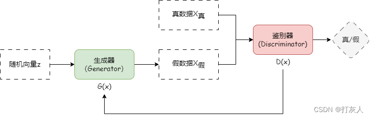
一个生成器和判别器博弈的过程。生成器生成假数据，然后将生成的假数据和真数据都输入判别器，判别器要判断出哪些是真的哪些是假的。判别器第一次判别出来的肯定有很大的误差，然后我们根据误差来优化判别器。现在判别器水平提高了，生成器生成的数据很难再骗过判别器了，所以我们得反过来优化生成器，之后生成器水平提高了，然后反过来继续训练判别器，判别器水平又提高了，再反过来训练生成器，就这样循环往复，直到达到纳什均衡。

（2）loss函数

生成器损失函数：

\[\begin{array}{l} L_G=H(1,D(G(z)))\\ \min_GV(G)=\mathbb{E}_{z\sim P_{Z}(z)}[log(1-D(G(z)))] \end{array}\]

G 代表生成网络，D 代表判别网络，H 代表交叉熵，z 是输入随机数据。\(D(G(z))\) 是对生成数据的判断概率，1代表数据绝对真实，0代表数据绝对虚假。\(H(1,D(G(z)))\)代表判断结果与1的距离。显然生成网络想取得良好的效果，那就要做到，让判别器将生成数据判别为真数据（即D(G(z))与1的距离越小越好)

判别器损失函数：

\[\begin{array}{l} L_D=H(1,D(x))+H(0,D(G(z)))\\ \max_{D}V(D)=\mathbb{E}_{x\sim P_{data}(x)}[log(D(x))]+\mathbb{E}_{z\sim P_{Z}(z)}[log(1-D(G(z)))] \end{array}\]

\(x\)是真实数据，这里要注意的是，\(H(1,D(x))\)代表真实数据与1的距离，\(H(0,D(G(z)))\)代表生成数据与0的距离。显然，识别网络要想取得良好的效果，那么就要做到，在它眼里，真实数据就是真实数据，生成数据就是虚假数据（即真实数据与1的距离小，生成数据与0的距离小)。

总体损失函数

\[\begin{array}{l} \min_G\max_{D}V(D,G)=\mathbb{E}_{x\sim P_{data}(x)}[log(D(x))]+\mathbb{E}_{z\sim P_{Z}(z)}[log(1-D(G(z)))] \end{array}\]

2、VAE

（1）VAE理解

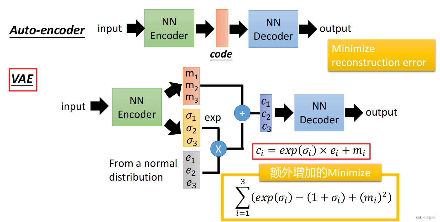
VAE = Variational Auto Encoder，变分自编码器。它能够学习一个函数/模型，使得输出数据的分布尽可能的逼近原始数据分布，其基本思路是：把一堆真实样本通过编码器网络变换成一个理想的数据分布，然后这个数据分布再传递给一个解码器网络，得到一堆生成样本，生成样本与真实样本足够接近的话，就训练出了一个VAE模型。

模型结构

简易理解

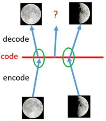
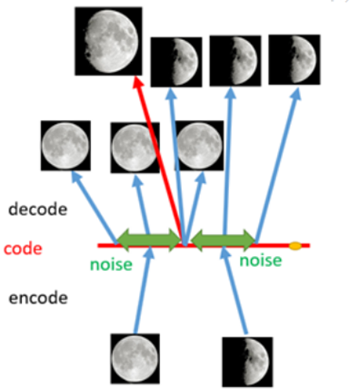
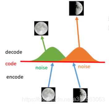
有两张训练图片一张全月图一张半月图，经过训练AE已经能无损地还原出两张图片，当我们在code空间两个图片编码点中间取一个点给解码器，预期能得到一张介于全月和半月之间的图片，但却得到了模糊无法辨认的乱码图，因为是单值编码，AE模型并没有找到code空间点与点之间迁移时的规律。重构输入的过程是否有噪声，是VAE和普通AE的区别之一。当我们引入噪声，如图：给两张图片编码的时候加上噪声，使得每张图片的编码点出现在绿色箭头所示范围内，模型训练时，绿色范围内的点都可能被采样到，解码器在训练时就能将绿色范围内的点尽可能还原成和原图相似的图片。从code中间取的介于全月和半月编码空间的点，就能得到两种图的过渡结果如3/4全月图。编码器加了噪声之后可以有效覆盖失真区域，但仍然不充分，如上图中黄色点仍未被覆盖，当把噪声无限拉长，对每一个样本来说，它的编码会覆盖整个编码空间，同时要保证在原编码附近编码的概率最高，离原编码点越远编码概率越低，这其实就是一个从离散到连续的过程，高斯分布能够描述这种编码特征，当然也可以用其他的分布类型来描述

（2）VAE推导

3、Flow-based

4、Diffusion

（1）简单推导

输入：\(x\) 输出：\(y\)

高斯分布：\(z\sim\mathcal{N}(0,1)\)

\(\beta\)：权重项，加噪的程度，正向过程加噪越来越多，0.0001到0.002，定义\(\alpha_t=1-\beta_t\)，\(\alpha\)越来越小，

加噪：\(x_t=\sqrt{\alpha_t}x_{t-1}+\sqrt{1-\alpha_t}z\)，越往后加的噪音越多

正向加噪过程：从\(x_{t-1}\)推\(x_t\)

通过添加高斯噪声将前向马尔可夫扩散过程 q

推导：

t时刻：\(x_t=\sqrt{\alpha_t}x_{t-1}+\sqrt{1-\alpha_t}z_1\)

t-1时刻：\(x_{t-1}=\sqrt{\alpha_{t-1}}x_{t-2}+\sqrt{1-\alpha_{t-1}}z_2\)

t-1时刻带入t时刻：

\[\begin{array}{l} x_t=\sqrt{\alpha_t}(\sqrt{\alpha_{t-1}}x_{t-2}+\sqrt{1-\alpha_{t-1}}z_2)+\sqrt{1-\alpha_t}z_1\\ x_t=\sqrt{\alpha_t\alpha_{t-1}}x_{t-2}+\sqrt{\alpha_t(1-\alpha_{t-1})}z_2+\sqrt{1-\alpha_t}z_2\\ x_t=\sqrt{\alpha_t\alpha_{t-1}}x_{t-2}+\sqrt{1-\alpha_t\alpha_{t-1}}z\\ \cdots\\ x_t=\sqrt{\overline{\alpha}}_tx_0+\sqrt{1-\overline{\alpha}_t}z_t \end{array}\]

其中\(\overline{\alpha}_t=\prod_{i=1}^T\alpha_i=\prod_{i=1}^T(1-\beta_i)\)

逆向过程：从\(x_{t}\)推\(x_{t-1}\)

贝叶斯公式：\(q(x_{t-1}\mid x_t,x_0)=q(x_t\mid x_{t-1},x_0)\frac{q(x_{t-1}\mid x_0)}{q(x_t\mid x_0)}\)

\[\begin{array}{l} q(x_t|x_{t-1},x_0)=\sqrt{\alpha_t}x_{t-1}+\sqrt{1-\alpha_t}z\sim\mathcal{N}(\sqrt{\alpha_t}x_{t-1},1-\alpha_t)\\ q(x_{t-1}|x_0)=\sqrt{\overline{\alpha}_{t-1}}x_0+\sqrt{1-\overline{\alpha}_{t-1}}z\sim\mathcal{N}(\sqrt{\overline{\alpha}_{t-1}}x_0,1-\overline{\alpha}_{t-1})\\ q(x_t|x_0)=\sqrt{\overline{\alpha}}_tx_0+\sqrt{1-\overline{\alpha}_t}z\sim\mathcal{N}(\sqrt{\overline{\alpha}}_tx_0,1-\overline{\alpha}_t) \end{array}\]

高斯分布公式：\(f(x)=\frac{1}{\sqrt{2\pi}}exp(-\frac{(x-\mu)^2}{2\sigma^2})\)

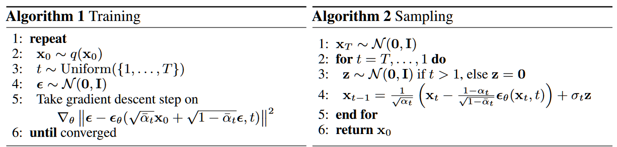
\[\begin{array}{l} q(x_{t-1}|x_t,x_0)=exp(-\frac{1}{2}(\frac{(x_{t}-\sqrt{\alpha_t}x_{t-1})^2}{\beta_t})+\frac{(x_{t-1}-\sqrt{\overline{\alpha}_{t-1}}x_0)^2}{1-\overline{\alpha}_{t-1}}-\frac{(x_{t}-\sqrt{\overline{\alpha}}_tx_0)^2}{1-\overline{\alpha}_t}))\\ q(x_{t-1}|x_t,x_0)=exp(-\frac{1}{2}((\frac{\alpha_t}{\beta_t}+\frac{1}{1-\overline{\alpha}_{t-1}})x_{t-1}^2)-(\frac{2\sqrt{\alpha_t}}{\beta_t}x_t+\frac{2\sqrt{\overline{\alpha}_{t-1}}}{1-\overline{\alpha}_{t-1}}x_0)x_{t-1}+C(x_t,x_0))\\ 高斯分布：exp(-\frac{(x-\mu)^2}{2\sigma^2})=exp(-\frac{1}{2}(\frac{1}{\sigma^2}x^2-\frac{2\mu}{\sigma^2}x+\frac{\mu^2}{\sigma^2}))对比得到均值和方差\\ \mu(x_t,x_0)=\frac{\sqrt{\alpha_t}(1-\overline{\alpha}_{t-1})}{1-\overline{\alpha}_{t}}x_t+\frac{\sqrt{\overline{\alpha}_{t-1}}\beta_t}{1-\overline{\alpha}_{t}}x_0\\ 由x_t=\sqrt{\overline{\alpha}}_tx_0+\sqrt{1-\overline{\alpha}_t}z_t\longrightarrow x_0=\frac{1}{\sqrt{\overline{\alpha}}_t}(x_t-\sqrt{1-\overline{\alpha}_t}z_t)带入\mu\\ \mu=\frac{1}{\sqrt{\alpha}_t}(x_t-\frac{\beta_t}{\sqrt{1-\overline{\alpha}_t}}z_t) \end{array}\]

我们用Unet学习的就是\(z_t\)

算法：

（2）概率论推导

正向加噪过程：从\(x_{t-1}\)推\(x_t\)

\[\begin{gathered} q(x_{1:T}|x_0)=\prod\limits_{t=1}^Tq(x_{t}|x_{t-1})\\ \text{其中}\quad q(x_{t}|x_{t-1})=\mathcal{N}(x_t|\sqrt{1-\beta_t}x_{t-1},\beta_tI)\\ \text{从而推导出：}\quad q(x_{t}|x_{0})=\mathcal{N}(x_t|\sqrt{\overline{\alpha}}_tx_0,(1-\overline{\alpha}_t)I) \end{gathered}\]

随着步数的增加最终变成高斯噪音

\[\begin{gathered} \beta<1\longrightarrow\lim\limits_{n\rightarrow\infty}\overline{\alpha}_t=0\\ \lim\limits_{t\rightarrow\infty}q(x_t)=\lim\limits_{t\rightarrow\infty}q(x_{t}|x_{0})=\mathcal{N}(0,I) \end{gathered}\]

逆向过程：从\(x_{t}\)推\(x_{t-1}\)

\[\begin{gathered} p_{\theta}(x_0)=\int p_{\theta}(x_{0:T})dx_{1:T}\\ p_{\theta}(x_{0:T})=p(x_T)\prod\limits_{t=1}^Tp_{\theta}(x_{t-1}|x_{t}) \end{gathered}\]

我们用 \(p_{\theta}(x_{t-1}\mid x_t)\) 去逼近 \(q(x_{t-1}\mid x_t)\)。

\[p_{\theta}(x_{t-1}|x_{t})=\mathcal{N}(x_{t-1}|\mu_{\theta}(x_t,t),\Sigma_{\theta}(x_t,t))\]

\(\mu_{\theta}\) 是可学习的，\(\Sigma_{\theta}\)是可学习的，但一般是\(\sigma_tI\)

（3）latent diffusion

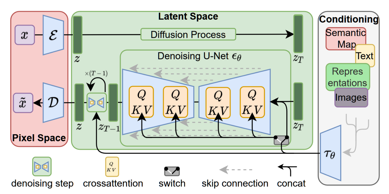
1.图像编码器将图像从像素空间（Pixel Space）压缩到更小维度的潜在空间（Latent Space），捕捉图像更本质的信息；

2.对潜在空间中的图片添加噪声，进行扩散过程（Diffusion Process）；

3.通过 CLIP 文本编码器将输入的描述语转换为去噪过程的条件（Conditioning）；

4.基于一些条件对图像进行去噪（Denoising）以获得生成图片的潜在表示，去噪步骤可以灵活地以文本、图像和其他形式为条件（以文本为条件即 text2img、以图像为条件即 img2img）；

5.图像解码器通过将图像从潜在空间转换回像素空间来生成最终图像

五、Transformer

0、Transformer基础

Attention

一个注意力函数可以描述为将 Query 与一组键值对（Key-Value）映射到输出，其中 Query、Key、Value 和输出都是向量。输出可以通过值的加权和而计算得出，在翻译任务中，Query 可以视为原语词向量序列，而 Key 和 Value 可以视为目标语词向量序列。一般的注意力机制可解释为计算 Query 和 Key 之间的相似性，并利用这种相似性确定 Query 和 Value 之间的注意力关系。

\[f(x)=\sum_i Attention(q,k_i)v_i\]

（1）Additivate Attention

\[\begin{array}{l} W_k\in\mathbb{R}^{h\times k},W_q\in\mathbb{R}^{h\times q},v\in\mathbb{R}^{h}\\ Attention(k,q)=v^T tanh(W_kk+W_qq) \end{array}\]

Query和Key纬度不一样，将Query和Key合并起来放入一个隐藏大小为h输出大小为1的单隐藏层MLP

（2）Scaled Dot-Product Attention

Query和Key纬度一样

\[\begin{array}{l} q,k\in \mathbb{R}^d,Attention(q,k)=\frac{<q,k>}{\sqrt{d}} \end{array}\]

向量版本：

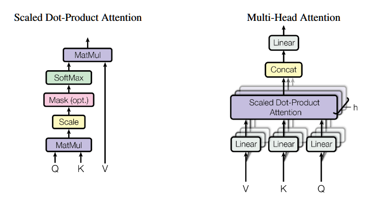
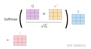
\[\begin{array}{l} Q\in\mathbb{R}^{n\times d},K\in\mathbb{R}^{m\times d},V\in\mathbb{R}^{m\times v}\\ 注意力分数：Attention(Q,K)=\frac{QK^T}{\sqrt{d}}\in\mathbb{R}^{m\times n}\\ 注意力池化：Attention(Q,K,V)=softmax(\frac{QK^T}{\sqrt{d_k}})V\in\mathbb{R}^{n\times v} \end{array}\]

注意力分数是Query和Key的相似度，注意力权重是注意力分数softmax的结果

Self-Attention

• Self-Attention

q：(查询) k：(键值) v：(值) x：tokens

one-head

\[Attention(Q,K,V)=softmax(\frac{QK^T}{\sqrt{d_k}})V\]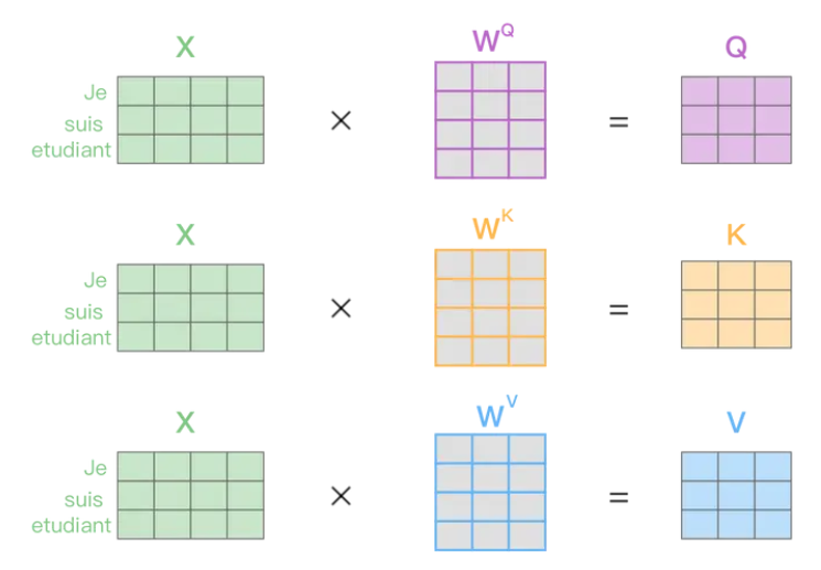

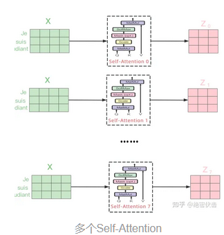
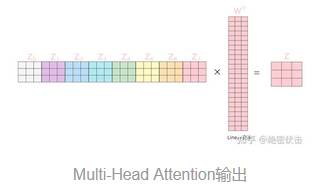
• Multi-Head Attention

\[\begin{array}{l} MuitiHead(Q,K,V)=Concate(head_1,\cdots,head_h)W^O\\ head_i=Attention(QW_i^Q,KW_i^K,VW_i^V) \end{array}\]

Cross-Attention

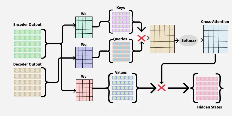
如何选 Q / K,V

• Q（Query）：代表“我想要的信息”。
  • 在你的任务里，就是 目标序列。
  • 因为 Q 是用来向外“打探”的。
• K,V（Key, Value）：代表“我能提供的信息”。
  • 在你的任务里，就是 辅助变量或外部因子。
  • K 用来和 Q 计算相似度，V 提供真正的值。

1、ViT

模型架构

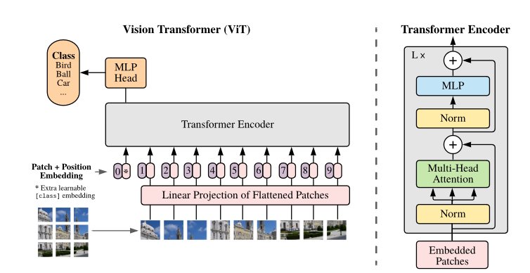
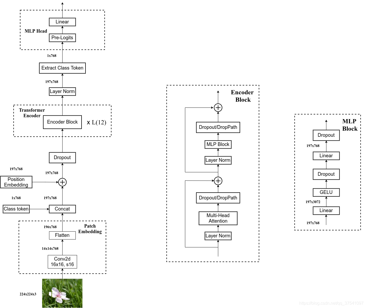
Patch Embedding

将图片变成若干个patch：利用size和步长相等的卷积实现，然后把长宽展平，每个patch就是一个token

如果是分类问题，需要加一个class token，[num_token+1, token_dim]

给token添加位置信息

Transformer Embedding

12个Transformer block堆叠，输入输出的是token（向量）序列，即二维矩阵[num_token, token_dim]

MPL Head

一个线性连接层，隐藏层是输入的四倍，用GELU激活

2、swin-Transformer

模型架构

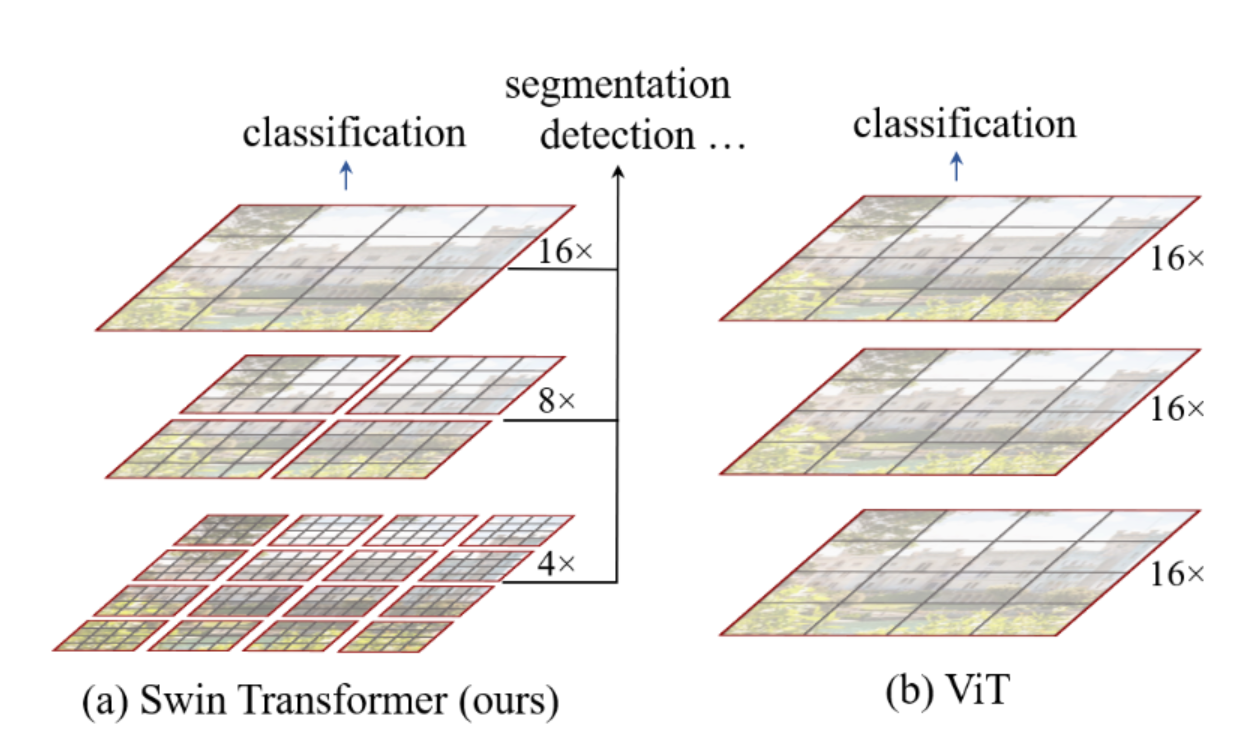
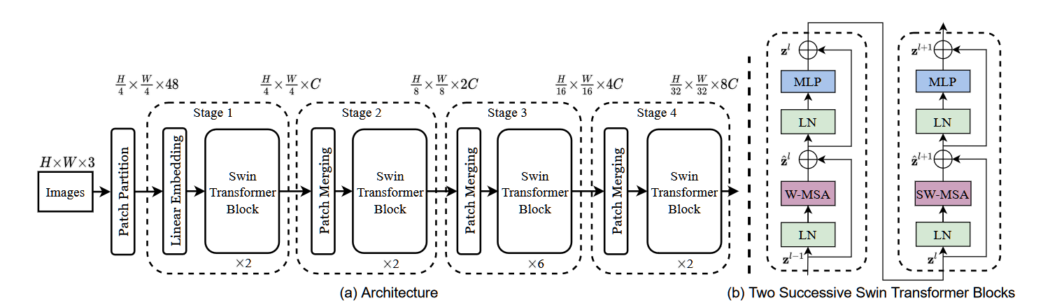
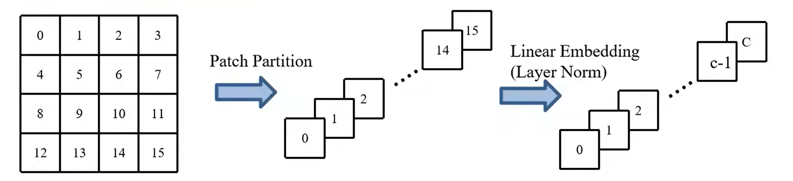
Patch Partiton&Linear Embeding

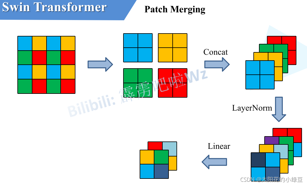
Patch Merging

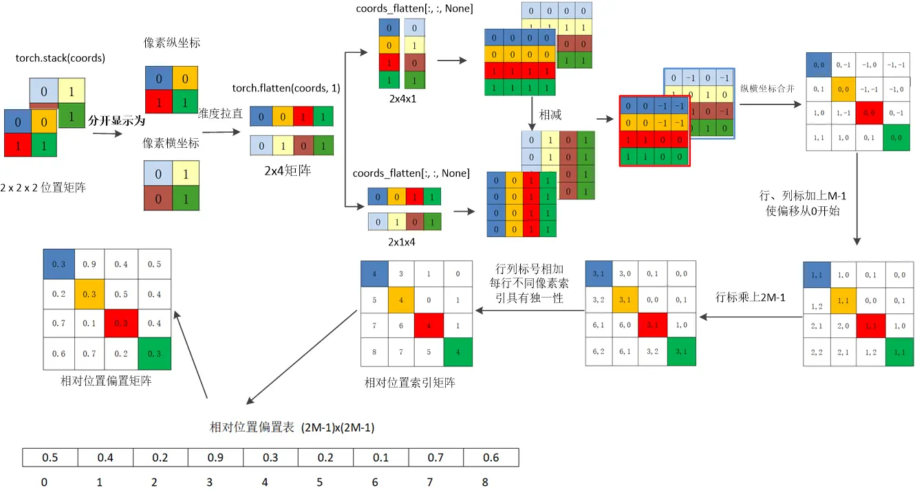
相对位置编码

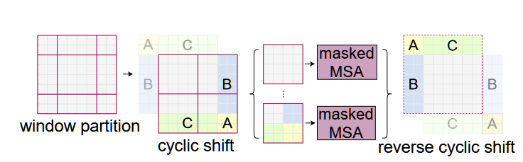
W-MSA&SW-MSA

六、GNN

1、Graph embedding

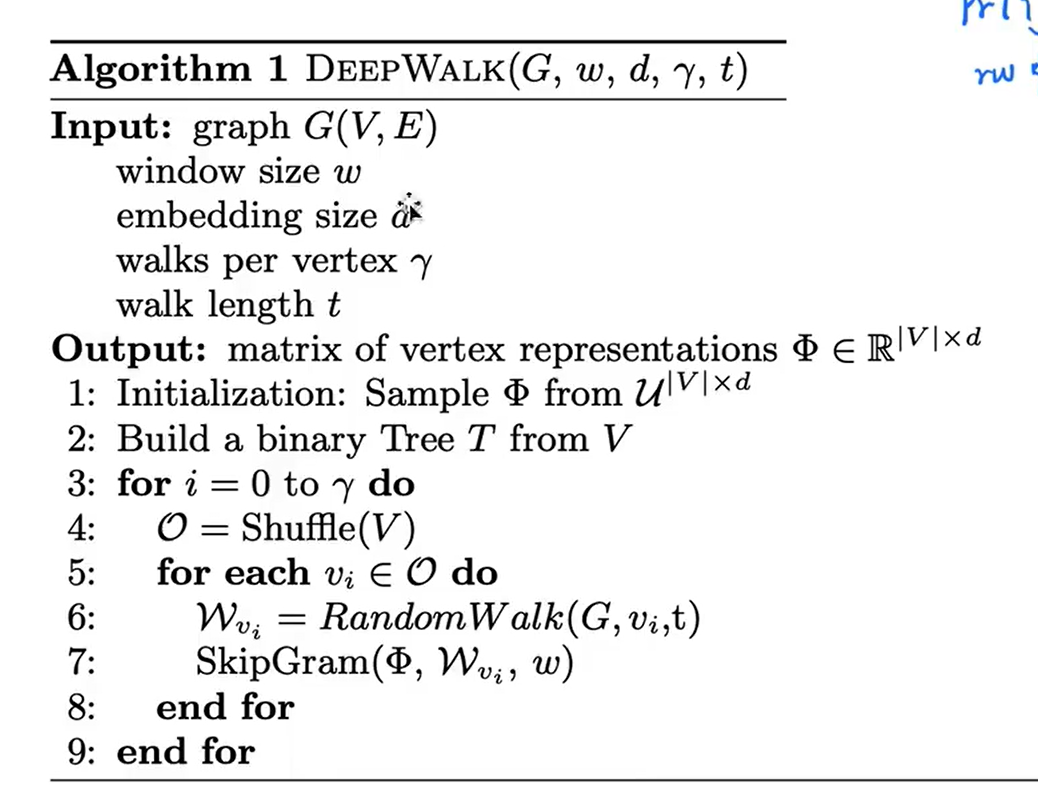
DeepWalk

LINE

一阶相似性：

距离相近的点的编码是相似的

顶点\(v_i\)，\(v_j\)的联合概率：\(p_1(v_i,v_j)=\frac{1}{1+exp(-u^T\cdot u_j)}\)

顶点\(v_i\)，\(v_j\)的经验概率：\(\hat{p}_1(i,j)=\frac{w_{i,j}}{W}\)

优化目标：

\[\begin{array}{l} D_{KL}(p||q)=\sum_{i=1}^n p(x_i)log(\frac{p(x_i)}{q(x_i)})\\ O_1=d(\hat{p_1},p_1)\\ O_1=-\sum_{(i,j)\in E}w_{i,j}\log p_1(v_i,v_j) \end{array}\]

二阶相似性：

共享节点邻居的点可能是相似的

二阶相似度计算的假设前提是：两个顶点共享其各自的一阶连接顶点，在这种情况下，顶点被看作是一种特定的「上下文」信息，因此每一个顶点都扮演了两个角色，即拥有两个embedding向量，一个是顶点本身的表示向量，一个是该点作为其他顶点的上下文顶点时的表示向量。

顶点的条件概率：

\[p_1(v_j\mid v_i)=\frac{exp(u^T_j\cdot u_i)}{\sum^{\lvert V\rvert}_{k=1} exp(-u^T\cdot u_j)}\]

顶点\(v_i\)，\(v_j\)的经验概率：\(\hat{p}_1(v_j\mid v_i)=\frac{w_{i,j}}{d_i}\)

优化目标：

\[\begin{array}{l} D_{KL}(p||q)=\sum_{i=1}^n p(x_i)log(\frac{p(x_i)}{q(x_i)})\\ O_2=\sum_{i\in V} \lambda_i d(\hat{p_2\cdot|v_i)},p_2(\cdot|v_i))\\ O_1=-\sum_{(i,j)\in E}w_{i,j}\log p_1(v_j\mid v_i) \end{array}\]

最后将1阶embedding和2阶embedding直接拼接

在度比较低的图效果不好，在度比较高的

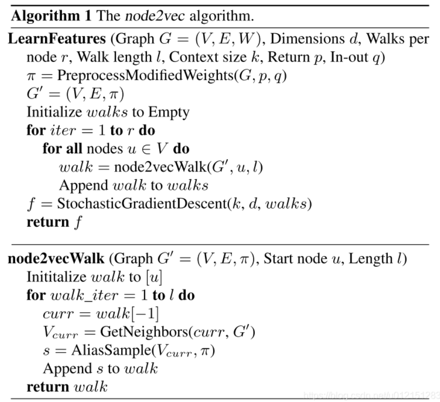
node2vec

同质性：距离相近的节点相似

结构等价性：结构相似的节点相似

Struc2vec

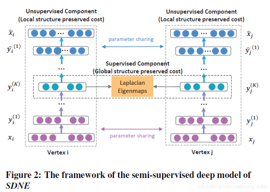
SDNE

用深度学习求embedding

\[\begin{array}{l} \mathcal{L}=\mathcal{L}_{2nd}+\alpha \mathcal{L}_{1st}+\nu \mathcal{L}_{reg}\\ =||(\hat{X}-X)B||^2+\alpha\sum^n_{i,j=1}s_{i,j}||y_i-y_j||^2_2+\nu \frac{1}{2}\sum^K_{k=1}(||W^{(k)}||^2_F+||\hat{W}^{(k)}||^2_F) \end{array}\]

2、MPNN(空域卷积)

图graph：

用G=(V, E)表示，V中元素为顶点（vertex），E中元素为边（edge）。图中边为无序对时为无向图，为有序对时为有向图

点vertex:

边edge:

度dgree:

邻接矩阵\(\widetilde{A}\)：

度矩阵\(\widetilde{D}\)：对角线是每个节点的度

\[\widetilde{D}_{ii}=\sum_j \widetilde{A}_{i,j}\]

一般的GNN

\[h_i=\sigma (W_1\cdot h_i+\sum_{{j\in \mathcal{N}_i}}W_2\cdot h_j)\]

GCN

\[h_i=\sigma(\widetilde{D}^{-\frac{1}{2}}\widetilde{A}\widetilde{D}^{-\frac{1}{2}}h_iW)\]

其中\(\widetilde{A}=A+I\)，\(\widetilde{D}^{-\frac{1}{2}}\)作用是归一化，\(h\)代表节点features

GraphSage

GAT

七、图文多模态模型

1、CLIP

clip 原理的极简版：

用图像编码器把图像编码成向量 a；
用文本编码器把文本编码成向量 b；
计算 a·b，
如果 a 和 b 来自一对儿配对的图和文字，则让 a·b 向 1 靠近；
如果 a 和 b 来自不配对儿的图和文字，则让 a·b 向 0 靠近；

clip 可以用来干啥：

根源用途：
    把图片和文字编码到同一空间，计算图像和文本的语义相似度；
扩展用途：
    1）图文搜索（根据图像搜索对应文本、或根据文本搜索对应图像）；
    2）协助完成相关的多模态任务（例如在 Stable Diffusion 里作为文本编码器）；
    3）作为评测工具（例如文生图任务中，计算生成图像与文本之间的相似度）。

训练

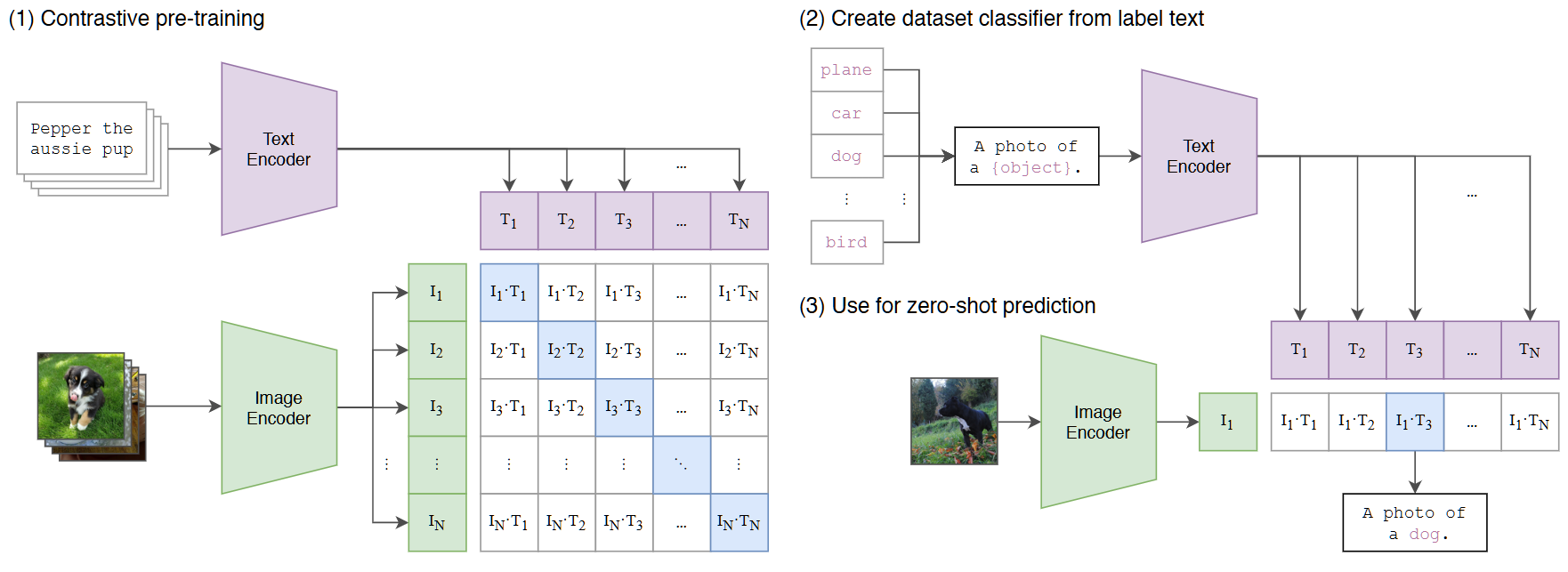
CLIP 模型主要由两个编码器组成：一个 文本编码器 和一个 图像编码器。在模型结构中，文本编码器通常采用 Transformer 架构（如 GPT-风格的 Transformer），而图像编码器则可以是 ResNet 或 Vision Transformer (ViT)。

训练数据由海量的图像–文本对组成，每一对数据都包含一张图片以及与其语义匹配的自然语言描述。训练时，输入的文本会首先经过文本编码器，得到对应的文本特征向量；输入的图像则会经过图像编码器，得到相应的图像特征向量。为了确保这两类特征能够在同一语义空间中对齐，CLIP会在输出端将二者映射到同一个向量空间。

在具体的优化过程中，模型会计算一个 相似度矩阵，矩阵的每个元素表示一个图像特征与一个文本特征之间的余弦相似度 (cosine similarity)。在一批数据 (batch) 内，正确的图像–文本对应该具有最高的相似度，而不相关的图文对则应当相对较低。训练目标就是通过 对比学习 (contrastive learning) 的方式，使得匹配的图像和文本在向量空间中的距离更近，而不匹配的距离更远。

这种优化通常采用 InfoNCE 损失函数。对于每一张图像，模型需要从 batch 中所有文本中“挑选”出唯一正确的描述；同理，对于每一段文本，也需要从 batch 中所有图像中找到唯一的配对。这相当于在每个 batch 内同时进行了一个 多分类任务：图像作为“查询”，文本作为“类别”，反之亦然。最终，通过最小化这个对比损失，模型能够有效地学习图像与语言之间的语义对齐关系。

1. CLIP 的任务

我们在一个 batch 里有 N 对图文。每张图像经过图像编码器 → 得到向量\(v_i\)；每段文本经过文本编码器 → 得到向量\(t_i\)。我们的目标是：让正确配对的\((v_i,t_i)\)相似度高，让不配对的相似度低。

1. 相似度计算

   余弦相似度：\(s_{ij} = \text{cosine\_sim}(v_i, t_j) = \frac{v_i \cdot t_j}{\Vert v_i\Vert \Vert t_j\Vert }\)

   这样就得到一个 N×N 的相似度矩阵：第i行表示第i张图像和所有文本的相似度。

2. InfoNCE 损失（以图像→文本为例）

   把“找正确的文本”当作一个分类问题。给定图像\(v_i\)，它和所有文本\(t_i\)计算相似度；正确答案是\(i=j\)。损失函数是交叉熵形式：

\[L_{\text{img→text}} = - \frac{1}{N} \sum_{i=1}^{N} \log \frac{\exp(s_{ii}/\tau)}{\sum_{j=1}^{N} \exp(s_{ij}/\tau)}\]

其中：\(s_{ii}\) 表示图像和它自己正确文本的相似度，\(\tau\)是一个温度系数，用来调节分布的“陡峭程度”。

1. 文本→图像方向

   同理，我们也能定义一个文本检索图像的损失：

\[L_{\text{text→img}} = - \frac{1}{N} \sum_{i=1}^{N} \log \frac{\exp(s_{ii}/\tau)}{\sum_{j=1}^{N} \exp(s_{ji}/\tau)}\]

1. 最终损失

   CLIP 同时优化两个方向：

\[L = \frac{1}{2}\Big( L_{\text{img→text}} + L_{\text{text→img}} \Big)\]

这样模型就学会了“图像找文本、文本找图像”两边都对齐。

推理

推理的基本流程

1. 输入：一张图像，或者一段文本，甚至是一组候选类别名字。
2. 编码：
   • 图像 → 图像编码器 → 向量\(v_i\)
   • 文本 → 文本编码器 → 向量\(t_i\)
3. 计算相似度：用余弦相似度比较\(v_i\)和\(t_i\)。
4. 输出结果：根据相似度来做分类、检索或匹配。

具体应用场景

(a) 图像分类（零样本分类）这样 CLIP 就能在没见过特定类别的情况下做分类。

• 给定一张图片 + 一些类别名字，比如 [“cat”, “dog”, “car”]。
• 用文本编码器把这些类别名字编码成向量。
• 再用图像编码器把图片编码成向量。
• 计算图片和每个类别向量的相似度，相似度最高的就是预测类别。

(b) 文本检索图像

• 输入一句话，比如 “a red sports car”。
• 把所有候选图片都编码成向量。
• 把文本编码成向量。
• 算相似度，把最相近的图片排在前面。

(c) 图像检索文本

• 输入一张图片。
• 把图片编码成向量。
• 和一堆文本描述做相似度匹配，找最合适的描述。

附录

1、手撕代码

self Attention

import math
import torch
import torch.nn as nn

class SelfAttention(nn.Module):
    def __init__(self, hidden_dim, p_dropout: float = 0.1) -> None:
        super().__init__()
        self.hidden_dim = hidden_dim

        # Q, K, V 线性映射（自注意力：来自同一个 X）
        self.q_proj = nn.Linear(hidden_dim, hidden_dim)
        self.k_proj = nn.Linear(hidden_dim, hidden_dim)
        self.v_proj = nn.Linear(hidden_dim, hidden_dim)

        # 注意力权重上的 dropout
        self.att_dropout = nn.Dropout(p_dropout)

        # 输出投影：把加权后的结果映射回 hidden_dim（保持接口一致）
        self.output_proj = nn.Linear(hidden_dim, hidden_dim)

    def forward(self, X, attention_mask=None):
        """
        自注意力（单头）
        X: (B, L, C)
        attention_mask: (B, L) 或已扩展成 (B, L, L)
                        0 表示遮挡，1 表示有效
        return: (B, L, C)
        """
        B, L, C = X.size()

        # 1) 得到 Q, K, V
        Q = self.q_proj(X)  # (B, L, C)
        K = self.k_proj(X)  # (B, L, C)
        V = self.v_proj(X)  # (B, L, C)

        # 2) 点积注意力分数：QK^T / sqrt(d_k)
        #    这里 d_k = C（单头，维度不拆）
        scores = (Q @ K.transpose(-1, -2)) / math.sqrt(C)   # (B, L, L)

        # 3) 应用 padding mask（如果提供）
        if attention_mask is not None:
            # 支持 (B, L) 或 (B, L, L)
            if attention_mask.dim() == 2:            # (B, L) -> (B, 1, L) 广播到 (B, L, L)
                scores = scores.masked_fill(attention_mask[:, None, :] == 0, float("-inf"))
            else:                                     # (B, L, L)
                scores = scores.masked_fill(attention_mask == 0, float("-inf"))

        # 4) softmax → dropout
        attn = torch.softmax(scores, dim=-1)          # (B, L, L)
        attn = self.att_dropout(attn)

        # 5) 加权求和：A @ V
        ctx = attn @ V                                 # (B, L, C)

        # 6) 输出投影
        out = self.output_proj(ctx)                    # (B, L, C)
        return out


# ===== 小测试 =====
if __name__ == "__main__":
    x = torch.randn(3, 5, 128)                # (B=3, L=5, C=128)
    # padding mask: 第 1 个样本最后两个位置是 pad；其它样本全有效
    pad_mask = torch.tensor([
        [1,1,1,0,0],
        [1,1,1,1,1],
        [1,1,1,1,1],
    ])                                        # (B, L)

    sa = SelfAttention(128)
    y = sa(x, attention_mask=pad_mask)
    print(y.shape)   # torch.Size([3, 5, 128])

Multi-Head Attention

import math
import torch
import torch.nn as nn

class MultiHeadAttention(nn.Module):
    def __init__(self, hidden_dim, nums_head) -> None:
        super().__init__()
        assert hidden_dim % nums_head == 0, "hidden_dim 必须能整除 nums_head"
        self.nums_head = nums_head
        self.head_dim = hidden_dim // nums_head
        self.hidden_dim = hidden_dim

        # Q, K, V 的线性映射
        self.q_proj = nn.Linear(hidden_dim, hidden_dim)
        self.k_proj = nn.Linear(hidden_dim, hidden_dim)
        self.v_proj = nn.Linear(hidden_dim, hidden_dim)

        # 注意力权重上的 dropout
        self.att_dropout = nn.Dropout(0.1)

        # 输出投影，把多头拼接后的结果映射回 hidden_dim
        self.output_proj = nn.Linear(hidden_dim, hidden_dim)

    def forward(self, X, attention_mask=None):
        """
        X: (B, L, C)
        attention_mask: (B, L) 或已扩展成 (B, num_heads, L, L) 0 表示要遮挡，1 表示有效位置
        """
        B, L, C = X.size()
        
        # 1. 线性映射得到 Q, K, V
        Q = self.q_proj(X)  # (B, L, C)
        K = self.k_proj(X)  # (B, L, C)
        V = self.v_proj(X)  # (B, L, C)

        # 2. 拆分成多头，并调整维度到 (B, H, L, D_h),H是head_num,D_h是head_dim
        q_state = Q.view(B, L, self.nums_head, self.head_dim).permute(0, 2, 1, 3)
        k_state = K.view(B, L, self.nums_head, self.head_dim).permute(0, 2, 1, 3)
        v_state = V.view(B, L, self.nums_head, self.head_dim).permute(0, 2, 1, 3)

        # 3. 计算注意力分数 (B, H, L, L)
        attention_weight = q_state @ k_state.transpose(-1, -2) / math.sqrt(self.head_dim)

        # 4. 应用 padding mask（如果提供）
        if attention_mask is not None:
            attention_weight = attention_weight.masked_fill(
                attention_mask == 0, float("-inf")
            )

        # 5. softmax 得到注意力分布
        attention_weight = torch.softmax(attention_weight, dim=-1)
        attention_weight = self.att_dropout(attention_weight)

        # 6. 加权求和得到上下文表示 (B, H, L, Dh)
        output_mid = attention_weight @ v_state

        # 7. 调整形状拼回 (B, L, C)
        output_mid = output_mid.transpose(1, 2).contiguous()
        output = output_mid.view(B, L, -1)

        # 8. 输出线性层
        output = self.output_proj(output)
        return output


# ==== Demo ====
# 构造一个 mask (3 个样本, 2 长度, 8 个头)
attention_mask = (torch.tensor([[0, 1], [0, 0], [1, 0]]).unsqueeze(1).unsqueeze(2).expand(3, 8, 2, 2))

x = torch.rand(3, 2, 128)
net = MultiHeadAttention(128, 8)
print(net(x, attention_mask).shape)  # (3, 2, 128)

Cross Attention

import math
import torch
import torch.nn as nn

class CrossAttention(nn.Module):
    def __init__(self, q_dim: int, nums_head: int, kv_dim: int | None = None, p_dropout: float = 0.1):
        super().__init__()
        kv_dim = kv_dim if kv_dim is not None else q_dim
        assert q_dim % nums_head == 0, "q_dim 必须能整除 nums_head"

        self.nums_head = nums_head
        self.head_dim  = q_dim // nums_head   # 统一用 q_dim 决定每头维度
        self.q_dim     = q_dim
        self.kv_dim    = kv_dim

        # Q 来自 X（q_dim -> q_dim），K/V 来自 M（kv_dim -> q_dim），这样切头后每头维度一致
        self.q_proj = nn.Linear(q_dim, q_dim)
        self.k_proj = nn.Linear(kv_dim, q_dim)
        self.v_proj = nn.Linear(kv_dim, q_dim)

        # 注意力权重 dropout
        self.att_dropout = nn.Dropout(p_dropout)
        # 输出投影，拼头后映射回 q_dim
        self.output_proj = nn.Linear(q_dim, q_dim)

    def forward(self, X: torch.Tensor, M: torch.Tensor, attention_mask: torch.Tensor | None = None):
        B, Lq, Cq = X.size()
        Bm, Lk, Ckv = M.size()
        assert B == Bm, "X 与 M batch 不一致"

        H, Dh = self.nums_head, self.head_dim

        # 1) 线性投影
        Q = self.q_proj(X)      # (B, Lq, q_dim)
        K = self.k_proj(M)      # (B, Lk, q_dim)
        V = self.v_proj(M)      # (B, Lk, q_dim)

        # 2) 切多头 -> (B, H, L, Dh)
        def split_heads(t, L):
            return t.view(B, L, H, Dh).permute(0, 2, 1, 3)
        q = split_heads(Q, Lq)   # (B,H,Lq,Dh)
        k = split_heads(K, Lk)   # (B,H,Lk,Dh)
        v = split_heads(V, Lk)   # (B,H,Lk,Dh)

        # 3) 注意力分数 (B,H,Lq,Lk)
        scores = (q @ k.transpose(-1, -2)) / math.sqrt(Dh)

        # 4) 应用 padding mask（如果提供）
        if attention_mask is not None:
            # 允许 (B, Lk) 或 (B, H, Lq, Lk)
            if attention_mask.dim() == 2:
                # (B, Lk) -> (B,1,1,Lk)，广播到 (B,H,Lq,Lk)
                mask = attention_mask[:, None, None, :].to(dtype=torch.bool)
            else:
                mask = attention_mask.to(dtype=torch.bool)
            scores = scores.masked_fill(~mask, float("-inf"))

        # 5) softmax & dropout
        attn = torch.softmax(scores, dim=-1)    # (B,H,Lq,Lk)
        attn = self.att_dropout(attn)

        # 6) 加权求和 → (B,H,Lq,Dh)
        ctx = attn @ v

        # 7) 拼回 (B,Lq,Cq) 并输出线性
        ctx = ctx.transpose(1, 2).contiguous().view(B, Lq, H * Dh)  # H*Dh = q_dim
        out = self.output_proj(ctx)                                  # (B,Lq,q_dim)
        return out


# ===== 简单测试 =====
if __name__ == "__main__":
    B, Lq, Lk = 2, 4, 5
    q_dim, kv_dim, H = 128, 256, 8
    x = torch.randn(B, Lq, q_dim)          # 查询序列（例如 decoder hidden）
    m = torch.randn(B, Lk, kv_dim)         # 上下文序列（例如 encoder outputs）

    # 针对 K/V 端的 padding mask：第一个样本末尾 2 个位置是 pad
    kv_pad = torch.tensor([
        [1,1,1,0,0],
        [1,1,1,1,1],
    ])  # (B, Lk)

    ca = CrossAttention(q_dim=q_dim, nums_head=H, kv_dim=kv_dim)
    y = ca(x, m, attention_mask=kv_pad)
    print(y.shape)  # torch.Size([2, 4, 128])

1. MLP

(1) Linear layer

Definition: A Linear layer is a basic layer type in deep learning frameworks such as PyTorch. It performs a linear transformation, that is, the output is the product of the input vector and the weight matrix plus a bias.

Characteristics:

• It performs only a linear transformation and contains no nonlinear activation function.
• It is a building block of FC layers or MLPs, because those usually append a nonlinear activation after the Linear layer.

(2) Activation functions

https://zhuanlan.zhihu.com/p/690848035

(3) MLP (Multi-Layer Perceptron)

Definition: MLP is short for multi-layer perceptron, a feedforward neural network that usually consists of an input layer, one or more hidden layers and an output layer. Neurons in each layer are fully connected to the neurons of the next layer. It is composed of several Linear layers and activation functions.

Characteristics:

• An MLP is a higher-level neural network structure containing multiple layers (input, hidden, output).
• Layers are fully connected (every neuron connects to every neuron of the next layer).
• It uses nonlinear activations (such as ReLU, Sigmoid, Tanh) to increase the network’s expressive power.

(4) KAN

2. CNN

0. Convolutional Neural Network Basics

Convolution

(1) Standard convolution

• Kernel size: the size of the convolution kernel.

• Stride: how far the kernels slide across the image.

• Padding: padding defines how the image borders are handled; convolution pads around the input boundary to keep the output the same size as the input image.

\[O=\frac{(I-Kernel\_size+2*Padding)}{Stride}+1\]

No padding, no strides

Arbitrary padding, no strides

Half padding, no strides

Full padding, no strides

No padding, strides

Padding, strides

Padding, strides (odd)

(2) Transposed convolution (deconvolution)

No padding, no strides, transposed

Arbitrary padding, no strides, transposed

Half padding, no strides, transposed

Full padding, no strides, transposed

No padding, strides, transposed

Padding, strides, transposed

Padding, strides, transposed (odd)

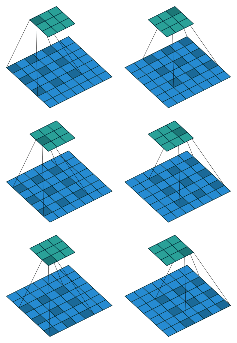
(3) Dilated convolution

No padding, no stride, dilation

Downsampling (pooling)

(1) Max pooling and average pooling

(2) Convolutional downsampling

Downsampling achieved by adjusting the kernel size, stride and padding.

(3) Interpolation downsampling

Downsampling performed with interpolation methods.

Upsampling

(1) Unpooling

Un-average pooling

First restore the original size, then place each value of the pooling result at the corresponding position of its original data region (the average replaces all values).

Un-max pooling

This requires recording the coordinates of the maximum activation value during pooling, and then during unpooling only the position of that maximum is activated while all other values are set to 0. Of course, this process is only an approximation, because during pooling the values other than the maximum are usually not 0 either.

(2) Deconvolution

Upsampling achieved by adjusting the kernel size, stride and padding.

(3) Sub-pixel convolution

(4) Interpolation

nearest, linear, bilinear, bicubic, trilinear, area, and so on.

1. AlexNet

In the first layer of AlexNet, the shape of the convolution window is 11×11. Because most images in ImageNet are more than ten times wider and taller than MNIST images, a larger convolution window is needed to capture the target. The convolution window shapes in the second layer are reduced to 5×5 and then 3×3. In addition, after the first, second and fifth convolution layers, a max pooling layer with a window shape of 3×3 and a stride of 2 is inserted.

AlexNet replaced the sigmoid activation with the simpler ReLU activation. On one hand, ReLU is cheaper to compute and does not need the complicated exponentiation that sigmoid requires. On the other hand, ReLU makes the model easier to train under different parameter initialization schemes. When the output of a sigmoid activation is very close to 0 or 1, the gradient in those regions is almost 0, so backpropagation can no longer update some model parameters. In contrast, the gradient of ReLU is always 1 in the positive region. Therefore, if the model parameters are not correctly initialized, the sigmoid function may yield a gradient of almost 0 in the positive region, preventing the model from being trained effectively.

2. VGG

The basic building block of a classic convolutional neural network is the following sequence:

1. A convolution layer with padding to preserve resolution;
2. A nonlinear activation, such as ReLU;
3. A pooling layer, such as max pooling.

The idea of using blocks first appeared in the VGG network from Oxford’s Visual Geometry Group. Using loops and subroutines, these repeated architectures are easy to implement in the code of any modern deep learning framework.

3. ResNet

(1) The residual idea

Suppose the original input is x and the desired ideal mapping is f(x). The part inside the dashed box in the left figure has to fit that mapping f(x) directly, whereas the part inside the dashed box in the right figure has to fit the residual mapping f(x)-x. The residual mapping is usually easier to optimize in practice. Taking the identity mapping as the ideal mapping f(x) we want to learn, we merely need to set the weights and biases of the weighted operation (such as an affine transform) above the dashed box in the right figure to 0, and then f(x) becomes the identity mapping. In practice, when the ideal mapping f(x) is extremely close to the identity mapping, the residual mapping also captures the subtle fluctuations of the identity mapping more easily.

(2) Residual block

The role of the \(1\times1\) convolution is to adjust the number of channels.

4. GoogLeNet (parallel)

In GoogLeNet the basic convolution block is called the Inception block.

The Inception block consists of four parallel paths. The first three paths use convolution layers with window sizes of 1×1, 3×3 and 5×5 to extract information at different spatial scales. The middle two paths apply 1×1 convolution to the input to reduce the number of channels and hence the model complexity. The fourth path uses a 3×3 max pooling layer followed by a 1×1 convolution layer to change the number of channels. All four paths use suitable padding so that the height and width of the input and output match; finally the outputs of the four paths are concatenated along the channel dimension to form the output of the Inception block. In an Inception block the hyper-parameter usually tuned is the number of output channels of each layer.

5. UNet

3. RNN

1. GRU

2. LSTM

3. Bidirectional RNN

4. Generative Models

1. GAN

(1) Model structure

A game between a generator and a discriminator. The generator produces fake data, and then both the generated fake data and the real data are fed to the discriminator, which must decide which is real and which is fake. The discriminator’s first judgments are bound to have a large error, and we optimize the discriminator based on that error. Now the discriminator has improved, and the data produced by the generator can hardly fool it any more, so we must optimize the generator in turn. After that the generator improves, so we go back to training the discriminator, which improves again, and then we train the generator again — and so on, cycling back and forth until a Nash equilibrium is reached.

(2) Loss functions

Generator loss:

\[\begin{array}{l} L_G=H(1,D(G(z)))\\ \min_GV(G)=\mathbb{E}_{z\sim P_{Z}(z)}[log(1-D(G(z)))] \end{array}\]

G denotes the generative network, D the discriminative network, H the cross entropy, and z the input random data. \(\displaystyle D(G(z))\) is the probability assigned to the generated data: 1 means the data is absolutely real, 0 means it is absolutely fake. \(H(1,D(G(z)))\) is the distance between the judgment and 1. Clearly, for the generator to do well, it must make the discriminator classify the generated data as real (that is, D(G(z)) should be as close to 1 as possible).

Discriminator loss:

\[\begin{array}{l} L_D=H(1,D(x))+H(0,D(G(z)))\\ \max_{D}V(D)=\mathbb{E}_{x\sim P_{data}(x)}[log(D(x))]+\mathbb{E}_{z\sim P_{Z}(z)}[log(1-D(G(z)))] \end{array}\]

\(x\) is the real data. Note here that \(H(1,D(x))\) is the distance between the real data and 1, while \(H(0,D(G(z)))\) is the distance between the generated data and 0. Clearly, for the discriminator to do well, in its eyes the real data must look real and the generated data must look fake (that is, the real data should be close to 1 and the generated data close to 0).

Overall loss function:

\[\begin{array}{l} \min_G\max_{D}V(D,G)=\mathbb{E}_{x\sim P_{data}(x)}[log(D(x))]+\mathbb{E}_{z\sim P_{Z}(z)}[log(1-D(G(z)))] \end{array}\]

2. VAE

(1) Understanding VAE

VAE = Variational Auto Encoder. It can learn a function/model that makes the distribution of the output data approach the original data distribution as closely as possible. The basic idea is: transform a set of real samples into an ideal data distribution through the encoder network, then pass that distribution to a decoder network to obtain a set of generated samples; if the generated samples are close enough to the real ones, a VAE model has been trained.

Model structure

An intuitive explanation

Suppose there are two training images, one full moon and one half moon. After training, an AE can already reconstruct both images losslessly. If we take a point in the code space halfway between the two encoded points and feed it to the decoder, we would expect an image between the full moon and the half moon, but we actually get a blurry, unrecognizable mess. Because the encoding is single-valued, the AE model has not learned the regularity of moving between points in code space. Whether there is noise in the process of reconstructing the input is one of the differences between a VAE and an ordinary AE. When we introduce noise, as in the figure: add noise when encoding the two images so that each image’s code lands somewhere within the range of the green arrow. During training, points inside the green region may be sampled, so the decoder learns to reconstruct points in the green region into images similar to the originals. Taking a point in code space midway between the full-moon and half-moon encodings then yields the transition between the two images, such as a three-quarter moon. Adding noise to the encoder effectively covers the distorted region, but it is still insufficient: the yellow point in the figure above remains uncovered. If the noise is stretched infinitely, then for each sample its code covers the entire code space, while the probability must be highest near the original code and lower the farther away the code is. This is in fact a process from discrete to continuous; a Gaussian distribution can describe this encoding characteristic, though other distribution types could be used as well.

(2) VAE derivation

3. Flow-based

4. Diffusion

(1) A simple derivation

Input: \(x\) Output: \(y\)

Gaussian distribution: \(z\sim\mathcal{N}(0,1)\)

\(\beta\): a weight term for the amount of noise added. In the forward process more and more noise is added, from 0.0001 to 0.002. Define \(\alpha_t=1-\beta_t\); \(\alpha\) gets smaller and smaller.

Add noise: \(x_t=\sqrt{\alpha_t}x_{t-1}+\sqrt{1-\alpha_t}z\); more noise is added as t grows.

Forward noising process: going from \(x_{t-1}\) to \(x_t\)

The forward Markov diffusion process q is built by adding Gaussian noise.

Derivation:

At step t: \(x_t=\sqrt{\alpha_t}x_{t-1}+\sqrt{1-\alpha_t}z_1\)

At step t-1: \(x_{t-1}=\sqrt{\alpha_{t-1}}x_{t-2}+\sqrt{1-\alpha_{t-1}}z_2\)

Substituting step t-1 into step t:

\[\begin{array}{l} x_t=\sqrt{\alpha_t}(\sqrt{\alpha_{t-1}}x_{t-2}+\sqrt{1-\alpha_{t-1}}z_2)+\sqrt{1-\alpha_t}z_1\\ x_t=\sqrt{\alpha_t\alpha_{t-1}}x_{t-2}+\sqrt{\alpha_t(1-\alpha_{t-1})}z_2+\sqrt{1-\alpha_t}z_2\\ x_t=\sqrt{\alpha_t\alpha_{t-1}}x_{t-2}+\sqrt{1-\alpha_t\alpha_{t-1}}z\\ \cdots\\ x_t=\sqrt{\overline{\alpha}}_tx_0+\sqrt{1-\overline{\alpha}_t}z_t \end{array}\]

where \(\overline{\alpha}_t=\prod_{i=1}^T\alpha_i=\prod_{i=1}^T(1-\beta_i)\)

Reverse process: going from \(x_{t}\) to \(x_{t-1}\)

Bayes’ formula: \(q(x_{t-1}\mid x_t,x_0)=q(x_t\mid x_{t-1},x_0)\frac{q(x_{t-1}\mid x_0)}{q(x_t\mid x_0)}\)

\[\begin{array}{l} q(x_t|x_{t-1},x_0)=\sqrt{\alpha_t}x_{t-1}+\sqrt{1-\alpha_t}z\sim\mathcal{N}(\sqrt{\alpha_t}x_{t-1},1-\alpha_t)\\ q(x_{t-1}|x_0)=\sqrt{\overline{\alpha}_{t-1}}x_0+\sqrt{1-\overline{\alpha}_{t-1}}z\sim\mathcal{N}(\sqrt{\overline{\alpha}_{t-1}}x_0,1-\overline{\alpha}_{t-1})\\ q(x_t|x_0)=\sqrt{\overline{\alpha}}_tx_0+\sqrt{1-\overline{\alpha}_t}z\sim\mathcal{N}(\sqrt{\overline{\alpha}}_tx_0,1-\overline{\alpha}_t) \end{array}\]

Gaussian formula: \(f(x)=\frac{1}{\sqrt{2\pi}}exp(-\frac{(x-\mu)^2}{2\sigma^2})\)

\[\begin{array}{l} q(x_{t-1}|x_t,x_0)=exp(-\frac{1}{2}(\frac{(x_{t}-\sqrt{\alpha_t}x_{t-1})^2}{\beta_t})+\frac{(x_{t-1}-\sqrt{\overline{\alpha}_{t-1}}x_0)^2}{1-\overline{\alpha}_{t-1}}-\frac{(x_{t}-\sqrt{\overline{\alpha}}_tx_0)^2}{1-\overline{\alpha}_t}))\\ q(x_{t-1}|x_t,x_0)=exp(-\frac{1}{2}((\frac{\alpha_t}{\beta_t}+\frac{1}{1-\overline{\alpha}_{t-1}})x_{t-1}^2)-(\frac{2\sqrt{\alpha_t}}{\beta_t}x_t+\frac{2\sqrt{\overline{\alpha}_{t-1}}}{1-\overline{\alpha}_{t-1}}x_0)x_{t-1}+C(x_t,x_0))\\ Gaussian: exp(-\frac{(x-\mu)^2}{2\sigma^2})=exp(-\frac{1}{2}(\frac{1}{\sigma^2}x^2-\frac{2\mu}{\sigma^2}x+\frac{\mu^2}{\sigma^2})); comparing terms gives the mean and variance\\ \mu(x_t,x_0)=\frac{\sqrt{\alpha_t}(1-\overline{\alpha}_{t-1})}{1-\overline{\alpha}_{t}}x_t+\frac{\sqrt{\overline{\alpha}_{t-1}}\beta_t}{1-\overline{\alpha}_{t}}x_0\\ From x_t=\sqrt{\overline{\alpha}}_tx_0+\sqrt{1-\overline{\alpha}_t}z_t\longrightarrow x_0=\frac{1}{\sqrt{\overline{\alpha}}_t}(x_t-\sqrt{1-\overline{\alpha}_t}z_t), substitute into \mu\\ \mu=\frac{1}{\sqrt{\alpha}_t}(x_t-\frac{\beta_t}{\sqrt{1-\overline{\alpha}_t}}z_t) \end{array}\]

What we learn with a UNet is \(z_t\).

Algorithm:

(2) A probability-theory derivation

Forward noising process: going from \(x_{t-1}\) to \(x_t\)

\[\begin{gathered} q(x_{1:T}|x_0)=\prod\limits_{t=1}^Tq(x_{t}|x_{t-1})\\ \text{where}\quad q(x_{t}|x_{t-1})=\mathcal{N}(x_t|\sqrt{1-\beta_t}x_{t-1},\beta_tI)\\ \text{hence}\quad q(x_{t}|x_{0})=\mathcal{N}(x_t|\sqrt{\overline{\alpha}}_tx_0,(1-\overline{\alpha}_t)I) \end{gathered}\]

As the number of steps grows the result eventually becomes Gaussian noise:

\[\begin{gathered} \beta<1\longrightarrow\lim\limits_{n\rightarrow\infty}\overline{\alpha}_t=0\\ \lim\limits_{t\rightarrow\infty}q(x_t)=\lim\limits_{t\rightarrow\infty}q(x_{t}|x_{0})=\mathcal{N}(0,I) \end{gathered}\]

Reverse process: going from \(x_{t}\) to \(x_{t-1}\)

\[\begin{gathered} p_{\theta}(x_0)=\int p_{\theta}(x_{0:T})dx_{1:T}\\ p_{\theta}(x_{0:T})=p(x_T)\prod\limits_{t=1}^Tp_{\theta}(x_{t-1}|x_{t}) \end{gathered}\]

We use \(p_{\theta}(x_{t-1}\mid x_{t})\) to approximate \(q(x_{t-1}\mid x_{t})\):

\[p_{\theta}(x_{t-1}|x_{t})=\mathcal{N}(x_{t-1}|\mu_{\theta}(x_t,t),\Sigma_{\theta}(x_t,t))\]

\(\mu_{\theta}\) is learnable and \(\Sigma_{\theta}\) is learnable too, but it is usually \(\sigma_tI\).

(3) Latent diffusion

1. An image encoder compresses the image from pixel space into a lower-dimensional latent space, capturing the more essential information of the image;
2. Noise is added to the image in latent space, performing the diffusion process;
3. A CLIP text encoder converts the input prompt into the condition for the denoising process (conditioning);
4. The image is denoised based on that condition to obtain the latent representation of the generated image. The denoising steps can be flexibly conditioned on text, images or other modalities (conditioned on text it is text2img, conditioned on an image it is img2img);
5. An image decoder converts the image from latent space back to pixel space to produce the final image.

5. Transformer

0. Transformer Basics

Attention

An attention function can be described as mapping a Query together with a set of key-value pairs to an output, where the Query, Keys, Values and output are all vectors. The output is computed as a weighted sum of the values. In a translation task, the Query can be seen as the sequence of source-language word vectors, while the Keys and Values can be seen as the sequence of target-language word vectors. In general, an attention mechanism can be interpreted as computing the similarity between the Query and the Keys and using that similarity to determine the attention relationship between the Query and the Values.

\[f(x)=\sum_i Attention(q,k_i)v_i\]

(1) Additive attention

\[\begin{array}{l} W_k\in\mathbb{R}^{h\times k},W_q\in\mathbb{R}^{h\times q},v\in\mathbb{R}^{h}\\ Attention(k,q)=v^T tanh(W_kk+W_qq) \end{array}\]

When the Query and Key have different dimensions, the Query and Key are combined and fed into a single-hidden-layer MLP with hidden size h and output size 1.

(2) Scaled dot-product attention

Here the Query and Key have the same dimension.

\[\begin{array}{l} q,k\in \mathbb{R}^d,Attention(q,k)=\frac{<q,k>}{\sqrt{d}} \end{array}\]

Vector form:

\[\begin{array}{l} Q\in\mathbb{R}^{n\times d},K\in\mathbb{R}^{m\times d},V\in\mathbb{R}^{m\times v}\\ attention scores: Attention(Q,K)=\frac{QK^T}{\sqrt{d}}\in\mathbb{R}^{m\times n}\\ attention pooling: Attention(Q,K,V)=softmax(\frac{QK^T}{\sqrt{d_k}})V\in\mathbb{R}^{n\times v} \end{array}\]

The attention scores are the similarities between the Query and the Keys, and the attention weights are the results of applying softmax to the attention scores.

Self-Attention

• Self-Attention

q: (query) k: (key) v: (value) x: tokens

One head:

\[Attention(Q,K,V)=softmax(\frac{QK^T}{\sqrt{d_k}})V\]

• Multi-Head Attention

\[\begin{array}{l} MuitiHead(Q,K,V)=Concate(head_1,\cdots,head_h)W^O\\ head_i=Attention(QW_i^Q,KW_i^K,VW_i^V) \end{array}\]

Cross-Attention

How to choose Q / K, V

• Q (Query): represents “the information I want”.
  • In your task, this is the target sequence.
  • Because the Query is what reaches out for information.
• K, V (Key, Value): represent “the information I can provide”.
  • In your task, these are the auxiliary variables or external factors.
  • The Key is used to compute similarity with the Query, and the Value provides the actual values.

1. ViT

Model architecture

Patch Embedding

The image is turned into several patches: this is done with a convolution whose kernel size equals its stride, and then the height and width are flattened; each patch is one token.

For classification problems a class token must be added, giving [num_token+1, token_dim].

Positional information is added to the tokens.

Transformer Embedding

12 Transformer blocks are stacked; the input and output are a sequence of tokens (vectors), that is, a two-dimensional matrix [num_token, token_dim].

MLP Head

A linear layer whose hidden layer is four times the input, activated with GELU.

2. Swin Transformer

Model architecture

Patch Partition & Linear Embedding

Patch Merging

Relative position encoding

W-MSA & SW-MSA

6. GNN

1. Graph embedding

DeepWalk

LINE

First-order proximity:

The encodings of nearby points are similar.

Joint probability of vertices \(v_i\) and \(v_j\): \(p_1(v_i,v_j)=\frac{1}{1+exp(-u^T\cdot u_j)}\)

Empirical probability of vertices \(v_i\) and \(v_j\): \(\hat{p}_1(i,j)=\frac{w_{i,j}}{W}\)

Optimization objective:

\[\begin{array}{l} D_{KL}(p||q)=\sum_{i=1}^n p(x_i)log(\frac{p(x_i)}{q(x_i)})\\ O_1=d(\hat{p_1},p_1)\\ O_1=-\sum_{(i,j)\in E}w_{i,j}\log p_1(v_i,v_j) \end{array}\]

Second-order proximity:

Points that share neighbors may be similar.

The assumption behind second-order similarity is that two vertices share their respective first-order neighbors; in that case a vertex is treated as a particular kind of “context” information. Every vertex therefore plays two roles and has two embedding vectors: one representing the vertex itself, and one representing the vertex when it acts as context for other vertices.

Conditional probability of a vertex:

\[p_1(v_j\mid v_i)=\frac{exp(u^T_j\cdot u_i)}{\sum^{\lvert V\rvert}_{k=1} exp(-u^T\cdot u_j)}\]

Empirical probability of vertices \(v_i\) and \(v_j\): \(\hat{p}_1(v_j\mid v_i)=\frac{w_{i,j}}{d_i}\)

Optimization objective:

\[\begin{array}{l} D_{KL}(p||q)=\sum_{i=1}^n p(x_i)log(\frac{p(x_i)}{q(x_i)})\\ O_2=\sum_{i\in V} \lambda_i d(\hat{p_2\cdot|v_i)},p_2(\cdot|v_i))\\ O_1=-\sum_{(i,j)\in E}w_{i,j}\log p_1(v_j\mid v_i) \end{array}\]

Finally the first-order and second-order embeddings are simply concatenated.

It performs poorly on graphs with low degree, and better on those with high degree.

node2vec

Homophily: nodes that are close to each other are similar.

Structural equivalence: nodes with similar structure are similar.

Struc2vec

SDNE

Using deep learning to obtain embeddings:

\[\begin{array}{l} \mathcal{L}=\mathcal{L}_{2nd}+\alpha \mathcal{L}_{1st}+\nu \mathcal{L}_{reg}\\ =||(\hat{X}-X)B||^2+\alpha\sum^n_{i,j=1}s_{i,j}||y_i-y_j||^2_2+\nu \frac{1}{2}\sum^K_{k=1}(||W^{(k)}||^2_F+||\hat{W}^{(k)}||^2_F) \end{array}\]

2. MPNN (spatial convolution)

Graph:

Represented as G=(V, E), where the elements of V are vertices and the elements of E are edges. When the edges are unordered pairs the graph is undirected; when they are ordered pairs it is directed.

Vertex:

Edge:

Degree:

Adjacency matrix \(\widetilde{A}\):

Degree matrix \(\widetilde{D}\): the diagonal holds the degree of each node.

\[\widetilde{D}_{ii}=\sum_j \widetilde{A}_{i,j}\]

A generic GNN

\[h_i=\sigma (W_1\cdot h_i+\sum_{{j\in \mathcal{N}_i}}W_2\cdot h_j)\]

GCN

\[h_i=\sigma(\widetilde{D}^{-\frac{1}{2}}\widetilde{A}\widetilde{D}^{-\frac{1}{2}}h_iW)\]

where \(\widetilde{A}=A+I\), \(\widetilde{D}^{-\frac{1}{2}}\) performs normalization, and \(h\) denotes the node features.

GraphSage

GAT

7. Image-Text Multimodal Models

1. CLIP

The minimal version of how CLIP works:

Encode an image into vector a with the image encoder;
encode text into vector b with the text encoder;
compute a·b;
if a and b come from a paired image and text, push a·b toward 1;
if a and b come from an unpaired image and text, push a·b toward 0;

What CLIP can be used for:

Core use:
    Encode images and text into the same space and compute their semantic similarity;
Extended uses:
    1) image-text search (find text from an image, or find images from text);
    2) assist other multimodal tasks (for example, acting as the text encoder in Stable Diffusion);
    3) act as an evaluation tool (for example, computing the similarity between a generated image and its prompt in text-to-image tasks).

Training

The CLIP model basically consists of two encoders: a text encoder and an image encoder. In the architecture, the text encoder usually adopts a Transformer (such as a GPT-style Transformer), while the image encoder can be a ResNet or a Vision Transformer (ViT).

The training data consists of a huge number of image-text pairs, each containing an image together with a natural language description that matches it semantically. During training, the input text first passes through the text encoder to obtain the corresponding text feature vector, and the input image passes through the image encoder to obtain the corresponding image feature vector. To ensure that these two types of features can be aligned in the same semantic space, CLIP maps both into a shared vector space at the output end.

In the actual optimization, the model computes a similarity matrix whose entries are the cosine similarities between one image feature and one text feature. Within a batch, the correct image-text pairs should have the highest similarity, while unrelated pairs should be relatively low. The training objective is to bring matching images and texts closer in vector space and push non-matching ones apart, through contrastive learning.

This optimization usually uses the InfoNCE loss. For every image, the model has to “pick out” the single correct description from all the texts in the batch; likewise, for every text it has to find its single matching image among all the images in the batch. This is equivalent to performing a multi-class classification task within each batch: the image acts as the “query” and the texts act as the “classes”, and vice versa. In the end, by minimizing this contrastive loss the model effectively learns the semantic alignment between images and language.

1. The CLIP task

Suppose a batch contains N image-text pairs. Every image passes through the image encoder to give a vector \(v_i\), and every text passes through the text encoder to give a vector \(t_i\). Our goal is to make the similarity of correctly paired \((v_i,t_i)\) high and that of unpaired pairs low.

1. Similarity computation

   Cosine similarity: \(s_{ij} = \text{cosine\_sim}(v_i, t_j) = \frac{v_i \cdot t_j}{\Vert v_i\Vert \Vert t_j\Vert }\)

   This yields an N×N similarity matrix: row i holds the similarities between image i and all texts.

2. InfoNCE loss (taking image→text as the example)

   Treat “finding the correct text” as a classification problem. Given image \(v_i\), its similarity is computed against all texts \(t_i\), and the correct answer is \(i=j\). The loss has the cross-entropy form:

\[L_{\text{img→text}} = - \frac{1}{N} \sum_{i=1}^{N} \log \frac{\exp(s_{ii}/\tau)}{\sum_{j=1}^{N} \exp(s_{ij}/\tau)}\]

where \(s_{ii}\) is the similarity between an image and its own correct text, and \(\tau\) is a temperature coefficient that adjusts how “steep” the distribution is.

1. The text→image direction

   Likewise we can define a text-to-image retrieval loss:

\[L_{\text{text→img}} = - \frac{1}{N} \sum_{i=1}^{N} \log \frac{\exp(s_{ii}/\tau)}{\sum_{j=1}^{N} \exp(s_{ji}/\tau)}\]

1. Final loss

   CLIP optimizes both directions at once:

\[L = \frac{1}{2}\Big( L_{\text{img→text}} + L_{\text{text→img}} \Big)\]

This way the model learns to align both “find the text from an image” and “find the image from text”.

Inference

The basic inference pipeline

1. Input: an image, or a piece of text, or even a set of candidate class names.
2. Encode:
   • image → image encoder → vector \(v_i\)
   • text → text encoder → vector \(t_i\)
3. Compute similarity: compare \(v_i\) and \(t_i\) with cosine similarity.
4. Output: perform classification, retrieval or matching based on the similarity.

Concrete application scenarios

(a) Image classification (zero-shot classification) — this way CLIP can classify without ever having seen the specific class.

• Given an image plus some class names, for example [“cat”, “dog”, “car”].
• Encode those class names into vectors with the text encoder.
• Encode the image into a vector with the image encoder.
• Compute the similarity between the image and each class vector; the highest similarity is the predicted class.

(b) Text-to-image retrieval

• Input a sentence, for example “a red sports car”.
• Encode all candidate images into vectors.
• Encode the text into a vector.
• Compute similarities and rank the closest images first.

(c) Image-to-text retrieval

• Input an image.
• Encode the image into a vector.
• Match it against a set of text descriptions by similarity and find the most suitable description.

Appendix

1. Hand-written Code

Self-Attention

import math
import torch
import torch.nn as nn

class SelfAttention(nn.Module):
    def __init__(self, hidden_dim, p_dropout: float = 0.1) -> None:
        super().__init__()
        self.hidden_dim = hidden_dim

        # Q, K, V linear projections (self-attention: all come from the same X)
        self.q_proj = nn.Linear(hidden_dim, hidden_dim)
        self.k_proj = nn.Linear(hidden_dim, hidden_dim)
        self.v_proj = nn.Linear(hidden_dim, hidden_dim)

        # dropout on the attention weights
        self.att_dropout = nn.Dropout(p_dropout)

        # output projection: map the weighted result back to hidden_dim (keeping the interface consistent)
        self.output_proj = nn.Linear(hidden_dim, hidden_dim)

    def forward(self, X, attention_mask=None):
        """
        Self-attention (single head)
        X: (B, L, C)
        attention_mask: (B, L) or already expanded to (B, L, L)
                        0 means masked, 1 means valid
        return: (B, L, C)
        """
        B, L, C = X.size()

        # 1) obtain Q, K, V
        Q = self.q_proj(X)  # (B, L, C)
        K = self.k_proj(X)  # (B, L, C)
        V = self.v_proj(X)  # (B, L, C)

        # 2) dot-product attention scores: QK^T / sqrt(d_k)
        #    here d_k = C (single head, the dimension is not split)
        scores = (Q @ K.transpose(-1, -2)) / math.sqrt(C)   # (B, L, L)

        # 3) apply the padding mask (if provided)
        if attention_mask is not None:
            # supports (B, L) or (B, L, L)
            if attention_mask.dim() == 2:            # (B, L) -> (B, 1, L), broadcast to (B, L, L)
                scores = scores.masked_fill(attention_mask[:, None, :] == 0, float("-inf"))
            else:                                     # (B, L, L)
                scores = scores.masked_fill(attention_mask == 0, float("-inf"))

        # 4) softmax -> dropout
        attn = torch.softmax(scores, dim=-1)          # (B, L, L)
        attn = self.att_dropout(attn)

        # 5) weighted sum: A @ V
        ctx = attn @ V                                 # (B, L, C)

        # 6) output projection
        out = self.output_proj(ctx)                    # (B, L, C)
        return out


# ===== small test =====
if __name__ == "__main__":
    x = torch.randn(3, 5, 128)                # (B=3, L=5, C=128)
    # padding mask: the last two positions of the first sample are pad; the others are fully valid
    pad_mask = torch.tensor([
        [1,1,1,0,0],
        [1,1,1,1,1],
        [1,1,1,1,1],
    ])                                        # (B, L)

    sa = SelfAttention(128)
    y = sa(x, attention_mask=pad_mask)
    print(y.shape)   # torch.Size([3, 5, 128])

Multi-Head Attention

import math
import torch
import torch.nn as nn

class MultiHeadAttention(nn.Module):
    def __init__(self, hidden_dim, nums_head) -> None:
        super().__init__()
        assert hidden_dim % nums_head == 0, "hidden_dim must be divisible by nums_head"
        self.nums_head = nums_head
        self.head_dim = hidden_dim // nums_head
        self.hidden_dim = hidden_dim

        # linear projections for Q, K, V
        self.q_proj = nn.Linear(hidden_dim, hidden_dim)
        self.k_proj = nn.Linear(hidden_dim, hidden_dim)
        self.v_proj = nn.Linear(hidden_dim, hidden_dim)

        # dropout on the attention weights
        self.att_dropout = nn.Dropout(0.1)

        # output projection, mapping the concatenated heads back to hidden_dim
        self.output_proj = nn.Linear(hidden_dim, hidden_dim)

    def forward(self, X, attention_mask=None):
        """
        X: (B, L, C)
        attention_mask: (B, L) or already expanded to (B, num_heads, L, L); 0 means masked, 1 means a valid position
        """
        B, L, C = X.size()
        
        # 1. linear projections to obtain Q, K, V
        Q = self.q_proj(X)  # (B, L, C)
        K = self.k_proj(X)  # (B, L, C)
        V = self.v_proj(X)  # (B, L, C)

        # 2. split into heads and reshape to (B, H, L, D_h),
        #    where H is the number of heads and D_h is the head dimension
        q_state = Q.view(B, L, self.nums_head, self.head_dim).permute(0, 2, 1, 3)
        k_state = K.view(B, L, self.nums_head, self.head_dim).permute(0, 2, 1, 3)
        v_state = V.view(B, L, self.nums_head, self.head_dim).permute(0, 2, 1, 3)

        # 3. compute the attention scores (B, H, L, L)
        attention_weight = q_state @ k_state.transpose(-1, -2) / math.sqrt(self.head_dim)

        # 4. apply the padding mask (if provided)
        if attention_mask is not None:
            attention_weight = attention_weight.masked_fill(
                attention_mask == 0, float("-inf")
            )

        # 5. softmax to obtain the attention distribution
        attention_weight = torch.softmax(attention_weight, dim=-1)
        attention_weight = self.att_dropout(attention_weight)

        # 6. weighted sum to obtain the context representation (B, H, L, Dh)
        output_mid = attention_weight @ v_state

        # 7. reshape and concatenate the heads back to (B, L, C)
        output_mid = output_mid.transpose(1, 2).contiguous()
        output = output_mid.view(B, L, -1)

        # 8. output linear layer
        output = self.output_proj(output)
        return output


# ==== Demo ====
# build a mask (3 samples, length 2, 8 heads)
attention_mask = (torch.tensor([[0, 1], [0, 0], [1, 0]]).unsqueeze(1).unsqueeze(2).expand(3, 8, 2, 2))

x = torch.rand(3, 2, 128)
net = MultiHeadAttention(128, 8)
print(net(x, attention_mask).shape)  # (3, 2, 128)

Cross Attention

import math
import torch
import torch.nn as nn

class CrossAttention(nn.Module):
    def __init__(self, q_dim: int, nums_head: int, kv_dim: int | None = None, p_dropout: float = 0.1):
        super().__init__()
        kv_dim = kv_dim if kv_dim is not None else q_dim
        assert q_dim % nums_head == 0, "q_dim must be divisible by nums_head"

        self.nums_head = nums_head
        self.head_dim  = q_dim // nums_head   # q_dim determines the per-head dimension
        self.q_dim     = q_dim
        self.kv_dim    = kv_dim

        # Q comes from X (q_dim -> q_dim), K/V come from M (kv_dim -> q_dim),
        # so that after splitting the heads each head has the same dimension
        self.q_proj = nn.Linear(q_dim, q_dim)
        self.k_proj = nn.Linear(kv_dim, q_dim)
        self.v_proj = nn.Linear(kv_dim, q_dim)

        # dropout on the attention weights
        self.att_dropout = nn.Dropout(p_dropout)
        # output projection, mapping back to q_dim after concatenating the heads
        self.output_proj = nn.Linear(q_dim, q_dim)

    def forward(self, X: torch.Tensor, M: torch.Tensor, attention_mask: torch.Tensor | None = None):
        B, Lq, Cq = X.size()
        Bm, Lk, Ckv = M.size()
        assert B == Bm, "X and M must have the same batch size"

        H, Dh = self.nums_head, self.head_dim

        # 1) linear projections
        Q = self.q_proj(X)      # (B, Lq, q_dim)
        K = self.k_proj(M)      # (B, Lk, q_dim)
        V = self.v_proj(M)      # (B, Lk, q_dim)

        # 2) split into heads -> (B, H, L, Dh)
        def split_heads(t, L):
            return t.view(B, L, H, Dh).permute(0, 2, 1, 3)
        q = split_heads(Q, Lq)   # (B,H,Lq,Dh)
        k = split_heads(K, Lk)   # (B,H,Lk,Dh)
        v = split_heads(V, Lk)   # (B,H,Lk,Dh)

        # 3) attention scores (B,H,Lq,Lk)
        scores = (q @ k.transpose(-1, -2)) / math.sqrt(Dh)

        # 4) apply the padding mask (if provided)
        if attention_mask is not None:
            # accepts (B, Lk) or (B, H, Lq, Lk)
            if attention_mask.dim() == 2:
                # (B, Lk) -> (B,1,1,Lk), broadcast to (B,H,Lq,Lk)
                mask = attention_mask[:, None, None, :].to(dtype=torch.bool)
            else:
                mask = attention_mask.to(dtype=torch.bool)
            scores = scores.masked_fill(~mask, float("-inf"))

        # 5) softmax & dropout
        attn = torch.softmax(scores, dim=-1)    # (B,H,Lq,Lk)
        attn = self.att_dropout(attn)

        # 6) weighted sum -> (B,H,Lq,Dh)
        ctx = attn @ v

        # 7) concatenate back to (B,Lq,Cq) and apply the output linear layer
        ctx = ctx.transpose(1, 2).contiguous().view(B, Lq, H * Dh)  # H*Dh = q_dim
        out = self.output_proj(ctx)                                  # (B,Lq,q_dim)
        return out


# ===== quick test =====
if __name__ == "__main__":
    B, Lq, Lk = 2, 4, 5
    q_dim, kv_dim, H = 128, 256, 8
    x = torch.randn(B, Lq, q_dim)          # query sequence (e.g. decoder hidden states)
    m = torch.randn(B, Lk, kv_dim)         # context sequence (e.g. encoder outputs)

    # padding mask for the K/V side: the last 2 positions of the first sample are pad
    kv_pad = torch.tensor([
        [1,1,1,0,0],
        [1,1,1,1,1],
    ])  # (B, Lk)

    ca = CrossAttention(q_dim=q_dim, nums_head=H, kv_dim=kv_dim)
    y = ca(x, m, attention_mask=kv_pad)
    print(y.shape)  # torch.Size([2, 4, 128])