深度学习——优化算法

发表于 2023/09/28

作者 Guanlong Ma

39 分钟 阅读

深度学习——优化算法

前言

所谓深度神经网络的优化算法，即用来更新神经网络参数，并使损失函数最小化的算法。优化算法对于深度学习非常重要，如果说网络参数初始化（模型迭代的初始点）能够决定模型是否收敛，那优化算法的性能则直接影响模型的训练效率。

了解不同优化算法的原理及其超参数的作用将使我们更有效的调整优化器的超参数，从而提高模型的性能。

本文的优化算法特指: 寻找神经网络上的一组参数 $\theta $，它能显著地降低损失函数 $J(\theta )$，该损失函数通常包括整个训练集上的性能评估和额外的正则化项。

本文损失函数、目标函数、代价函数不严格区分定义。

一，梯度下降优化算法

1.1，随机梯度下降 SGD

梯度下降法是最基本的一类优化器，目前主要分为三种梯度下降法：标准梯度下降法(GD, Gradient Descent)，随机梯度下降法(SGD, Stochastic Gradient Descent)及批量梯度下降法(BGD, Batch Gradient Descent)。

深度学习项目中的 SGD 优化一般默认指批量梯度下降法。其算法描述如下:

输入和超参数: $\eta$ 全局学习率
计算梯度：$g_t = \nabla_\theta J(\theta_{t-1})$
更新参数：$\theta_t = \theta_{t-1} - \eta \cdot g_t$

SGD 优化算法是最经典的神经网络优化方法，虽然收敛速度慢，但是收敛效果比较稳定。

下图1展现了随机梯度下降算法的梯度搜索轨迹示意图。可以看出由于梯度的随机性质，梯度搜索轨迹要很嘈杂（动荡现象）。

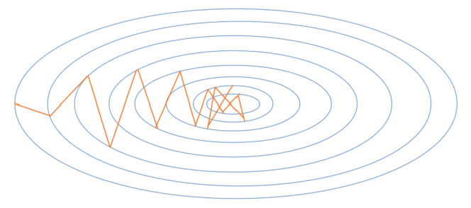
因此，在实际应用中，随机梯度下降 SGD 法必须和动态学习率方法结合起来使用，否则使用固定学习率 + SGD的组合会使得模型收敛过程变得更复杂。

1.2，动量 Momentum

虽然随机梯度下降仍然是非常受欢迎的优化方法，但其学习过程有时会很慢且其梯度更新方向完全依赖于当前 batch 样本数据计算出的梯度，因而十分不稳定，因为数据可能有噪音。

受启发于物理学研究领域研究，基于动量 Momentum (Polyak, 1964) 的 SGD 算法用于改善参数更新时可能产生的振荡现象。动量算法旨在加速学习，特别是处理高曲率、小但一致的梯度，或是带噪声的梯度。两种算法效果对比如下图 2所示。

花书中对动量算法对目的解释是，解决两个问题: Hessian 矩阵的病态条件和随机梯度的方差。更偏学术化一点。

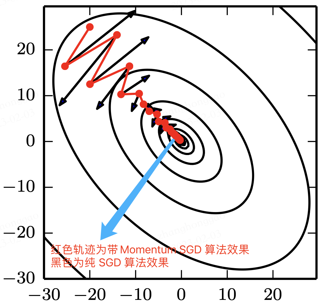
Momentum 算法的通俗理解就是，其模拟了物体运动时的惯性，即更新参数的时候会同时结合过去以及当前 batch 的梯度。算法在更新的时候会一定程度上保留之前更新的方向，同时利用当前 batch 的梯度微调最终的更新方向。这样一来，可以在一定程度上增加稳定性，从而学习地更快，并且还有一定摆脱局部最优的能力。

下图3展现了动量算法的前进方向。

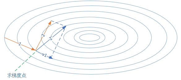
第一次的梯度更新完毕后，会记录 $v1$ 的动量值。在“求梯度点”进行第二次梯度检查时，得到2号方向，与 $v1$ 的动量组合后，最终的更新为 2’ 方向。这样一来，由于有 $v1$ 的存在，会迫使梯度更新方向具备“惯性”，从而可以减小随机样本造成的震荡。

Momentum 算法描述如下:

1，输入和参数:

$\eta$ - 全局学习率
$\alpha$ - 动量参数，一般取值为 0.5, 0.9, 0.99，取 0，则等效于常规的随机梯度下降法，其控制动量信息对整体梯度更新的影响程度。
$v_t$ - 当前时刻的动量，初值为 0。

2，算法计算过程：

计算梯度：$g_t = \nabla_\theta J(\theta_{t-1})$
计算速度更新：$v_t = \alpha \cdot v_{t-1} + \eta \cdot g_t$ (公式1)
更新参数：$\theta_t = \theta_{t-1} - v_t$ (公式2)

注意，这里的公式1和公式2和花书上的公式形式上略有不同，但其最终结果是相同的。本文给出的手工推导迭代公式，来源文章 15.2 梯度下降优化算法。

通过推导参数更新迭代公式，更容易理解算法，根据算法公式(1)(2)，以$W$参数为例，有：

\[v_0 = 0\]
\[dW_0 = \nabla J(w)\]
\[v_1 = \alpha v_0 + \eta \cdot dW_0 = \eta \cdot dW_0\]
\[W_1 = W_0 - v_1=W_0 - \eta \cdot dW_0\]
\[dW_1 = \nabla J(w)\]
\[v_2 = \alpha v_1 + \eta dW_1\]
\[W_2 = W_1 - v_2 = W_1 - (\alpha v_1 +\eta dW_1) = W_1 - \alpha \cdot \eta \cdot dW_0 - \eta \cdot dW_1\]
\[dW_2 = \nabla J(w)\]
\[v_3=\alpha v_2 + \eta dW_2\]
\[W_3 = W_2 - v_3=W_2-(\alpha v_2 + \eta dW_2) = W_2 - \alpha^2 \eta dW_0 - \alpha \eta dW_1 - \eta dW_2\]

可以看出与普通 SGD 的算法 $W_3 = W_2 - \eta dW_2$ 相比，动量法不但每次要减去当前梯度，还要减去历史梯度$W_0, W_1$ 乘以一个不断减弱的因子$\alpha$、$\alpha^2$，因为$\alpha$小于1，所以$\alpha^2$比$\alpha$小，$\alpha^3$比$\alpha^2$小。这种方式的学名叫做指数加权平均。

在实际模型训练中，SGD 和动量法的比较如下表所示。

实验效果对比图来源于资料 1。

算法	损失函数和准确率
SGD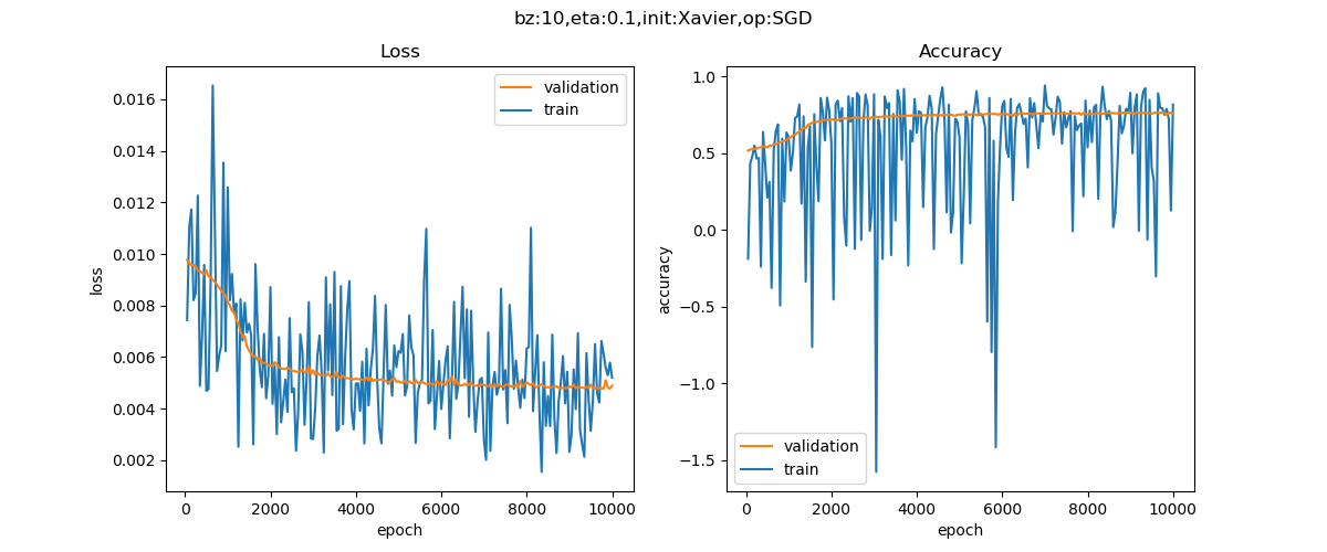
Momentum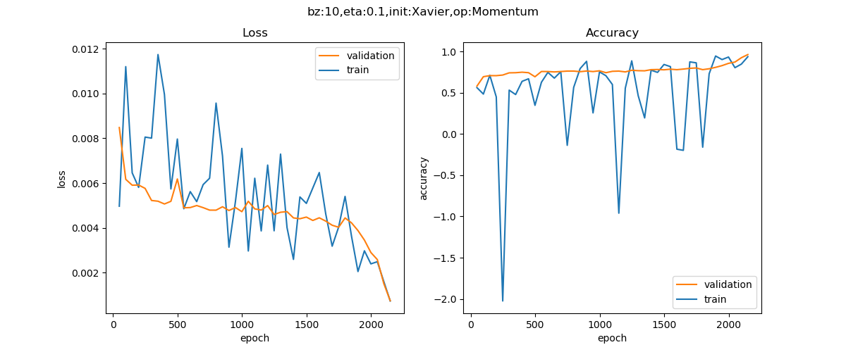

从上表的对比可以看出，同一个深度模型，普通随机梯度下降法的曲线震荡很严重，且经过 epoch=10000 次也没有到达预定 0.001 的损失值；但动量算法经过 2000 个 epoch 就迭代结束。

1.3，Nesterov 动量

受 Nesterov 加速梯度算法 (Nesterov, 1983, 2004) 启发，Sutskever et al. (2013) 提出了动量算法的一个变种，Nesterov 动量随机下降法（NAG ，英文全称是 Nesterov Accelerated Gradient，或者叫做 Nesterov Momentum 。

Nesterov 动量随机梯度下降方法是在上述动量梯度下降法更新梯度时加入对当前梯度的校正，简单解释就是往标准动量方法中添加了一个校正因子。

NAG 算法描述如下:

1，输入和参数：

$\eta$ - 全局学习率
$\alpha$ - 动量参数，缺省取值 0.9
$v$ - 动量，初始值为0

2，算法计算过程：

参数临时更新：$\hat \theta = \theta_{t-1} - \alpha \cdot v_{t-1}$
网络前向传播计算：$f(\hat \theta)$
计算梯度：$g_t = \nabla_{\hat\theta} J(\hat \theta)$
计算速度更新：$v_t = \alpha \cdot v_{t-1} + \eta \cdot g_t$
更新参数：$\theta_t = \theta_{t-1} - v_t$

1.4，代码实践

Pytorch 框架中把普通 SGD、Momentum 算法和 Nesterov Momentum 算法的实现结合在一起了，对应的类是 torch.optim.SGD。注意，其更新公式与其他框架略有不同，其中 $p$、$g$、$v$、$\mu$ 表示分别是参数、梯度、速度和动量。

\[\begin{align} v_{t+1} &= \mu * v_{t} + g_{t+1} \nonumber \\ p_{t+1} &= p_{t} - \text{lr} * v_{t+1} \nonumber \\ &= p_{t} - \text{lr} * \mu * v_{t} - \text{lr} * g_{t+1} \nonumber \end{align}\]

  
# 和源码比省略了部分不常用参数
class torch.optim.SGD(params, lr=required, momentum=0, dampening=0,
                 weight_decay=0, nesterov=False)

1，功能解释：

可实现 SGD 优化算法、带动量 SGD 优化算法、带 NAG(Nesterov accelerated gradient)动量 SGD 优化算法，并且均可拥有 weight_decay 项。

2，参数解释：

params(iterable): 参数组(参数组的概念参考优化器基类: Optimizer)，即优化器要管理的那部分参数。
lr(float): 初始学习率，可按需随着训练过程不断调整学习率。
momentum(float): 动量因子，通常设置为 0.9，0.8。
weight_decay(float): 权值衰减系数，也就是 L2 正则项的系数。
nesterov(bool)- bool 选项，是否使用 NAG(Nesterov accelerated gradient)。

训练模型时常用配置如下:

  
torch.optim.SGD(lr=0.02, momentum=0.9, weight_decay=0.0001)

二，自适应学习率算法

神经网络研究员早就意识到学习率肯定是难以设置的超参数之一，因为它对深度学习模型的性能有着显著的影响。

2.1，AdaGrad

在 AdaGrad (Duchi et al., 2011) 提出之前，我们对于所有的参数使用相同的学习率进行更新，它是第一个自适应学习率算法，通过所有梯度历史平方值之和的平方根，从而使得步长单调递减。它根据自变量在每个维度的梯度值的大小来调整各个维度上的学习率，从而避免统一的学习率难以适应所有维度的问题。

AdaGrad 法根据训练轮数的不同，对学习率进行了动态调整。具体表现在，对低频出现的参数进行大的更新（快速下降的学习率），对高频出现的参数进行小的更新（相对较小的下降学习率）。因此，他很适合于处理稀疏数据。

AdaGrad 算法描述如下:

1，输入和参数

$\eta$ - 全局学习率
$\epsilon$ - 用于数值稳定的小常数，建议缺省值为1e-6
$r=0$ 初始值

2，算法计算过程：

计算梯度：$g_t = \nabla_\theta J(\theta_{t-1})$
累计平方梯度：$r_t = r_{t-1} + g_t \odot g_t$
计算梯度更新：$\Delta \theta = {\eta \over \epsilon + \sqrt{r_t}} \odot g_t$(和动手学深度学习给出的学习率调整公式形式不同)
更新参数：$\theta_t=\theta_{t-1} - \Delta \theta$

$\odot$ 按元素相乘，开方、除法和乘法的运算都是按元素运算的。这些按元素运算使得目标函数自变量中每个元素都分别拥有自己的学习率。

AdaGrad 总结：在凸优化背景中，AdaGrad 算法具有一些令人满意的理论性质。但是，经验上已经发现，对于训练深度神经网络模型而言，从训练开始时积累梯度平方会导致有效学习率过早和过量的减小。AdaGrad 在某些深度学习模型上效果不错，但不是全部。

Pytorch 框架中 AdaGrad 优化器:

  
class torch.optim.Adagrad(params, lr=0.01, lr_decay=0, weight_decay=0, initial _accumulator_value=0)

2.2，RMSProp

RMSProp（Root Mean Square Prop），均方根反向传播。

RMSProp 算法 (Hinton, 2012) 和 AdaGrad 算法的不同在于， RMSProp算法使用了小批量随机梯度按元素平方的指数加权移动平均来调整学习率。

RMSProp 算法描述如下:

1，输入和参数：

$\eta$ - 全局学习率，建议设置为0.001
$\epsilon$ - 用于数值稳定的小常数，建议缺省值为1e-8
$\alpha$ - 衰减速率，建议缺省取值0.9
$r$ - 累积变量矩阵，与$\theta$尺寸相同，初始化为0

2，算法计算过程（计算梯度和更新参数公式和 AdaGrad 算法一样）：

累计平方梯度：$r = \alpha \cdot r + (1-\alpha)(g_t \odot g_t)$
计算梯度更新：$\Delta \theta = {\eta \over \sqrt{r + \epsilon}} \odot g_t$

RMSProp 总结：经验上，RMSProp 已被证明是一种有效且实用的深度神经网络优化算法。目前，它是深度学习从业者经常采用的优化方法之一。其初始学习率设置为 0.01 时比较理想。

Pytorch 框架中 RMSprop 优化器:

  
class torch.optim.RMSprop(params, lr=0.01, alpha=0.99, eps=1e- 08, weight_decay=0, momentum=0, centered=False)

2.3，AdaDelta

AdaDelta 法也是对 AdaGrad 法的一种改进，它旨在解决深度模型训练后期，学习率过小问题。相比计算之前所有梯度值的平方和，AdaDelta 法仅计算在一个大小为 $w$ 的时间区间内梯度值的累积和。

RMSProp 算法计算过程如下:

1，参数定义：

Adadelta 没有学习率参数。相反，它使用参数本身的变化率来调整学习率。
$s$ - 累积变量，初始值 0

2，算法计算过程:

计算梯度：$g_t = \nabla_\theta J(\theta_{t-1})$
累积平方梯度：$s_t = \alpha \cdot s_{t-1} + (1-\alpha) \cdot g_t \odot g_t$
计算梯度更新：$\Delta \theta = \sqrt{r_{t-1} + \epsilon \over s_t + \epsilon} \odot g_t$
更新梯度：$\theta_t = \theta_{t-1} - \Delta \theta$
更新变化量：$r = \alpha \cdot r_{t-1} + (1-\alpha) \cdot \Delta \theta \odot \Delta \theta$

Pytorch 框架中 Adadelta 优化器:

  
class torch.optim.Adadelta(params, lr=1.0, rho=0.9, eps=1e- 06, weight_decay=0)

2.4，Adam

Adam (Adaptive Moment Estimation，Kingma and Ba, 2014) 是另一种学习率自适应的优化算法，相当于 RMSProp + Momentum 的效果，即动量项的 RMSprop 算法。

Adam 算法在 RMSProp 算法基础上对小批量随机梯度也做了指数加权移动平均。和 AdaGrad 算法、RMSProp 算法以及 AdaDelta 算法一样，目标函数自变量中每个元素都分别拥有自己的学习率。

Adam 算法计算过程如下:

1，参数定义：

$t$ - 当前迭代次数
$\eta$ - 全局学习率，建议缺省值为0.001
$\epsilon$ - 用于数值稳定的小常数，建议缺省值为1e-8
$\beta_1, \beta_2$ - 矩估计的指数衰减速率，$\in[0,1)$，建议缺省值分别为0.9和0.999

2，算法计算过程:

计算梯度：$g_t = \nabla_\theta J(\theta_{t-1})$
计数器加一：$t=t+1$
更新有偏一阶矩估计：$m_t = \beta_1 \cdot m_{t-1} + (1-\beta_1) \cdot g_t$
更新有偏二阶矩估计：$v_t = \beta_2 \cdot v_{t-1} + (1-\beta_2)(g_t \odot g_t)$
修正一阶矩的偏差：$\hat m_t = m_t / (1-\beta_1^t)$
修正二阶矩的偏差：$\hat v_t = v_t / (1-\beta_2^t)$
计算梯度更新：$\Delta \theta = \eta \cdot \hat m_t /(\epsilon + \sqrt{\hat v_t})$
更新参数：$\theta_t=\theta_{t-1} - \Delta \theta$

从上述公式可以看出 Adam 使用指数加权移动平均值来估算梯度的动量和二次矩，即使用了状态变量 $m_t、v_t$。

怎么理解 Adam 算法？

首先，在 Adam 中，动量直接并入了梯度一阶矩(指数加权)的估计。将动量加入 RMSProp 最直观的方法是将动量应用于缩放后的梯度。结合缩放的动量使用没有明确的理论动机。其次，Adam 包括偏置修正，修正从原点初始化的一阶矩(动量项)和(非中心的)二阶矩的估计。RMSProp 也采用了(非中心的)二阶矩估计，然而缺失了修正因子。因此，不像 Adam，RMSProp 二阶矩估计可能在训练初期有很高的偏置。 Adam 通常被认为对超参数的选择相当鲁棒，尽管学习率有时需要从建议的默认修改。

初学者看看公式就行，这段话我也是摘抄花书，目前没有很深入理解。

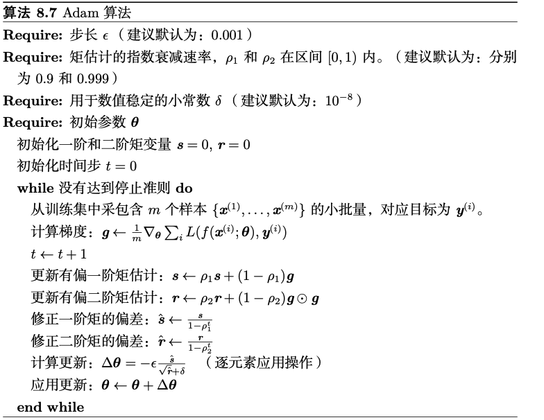
Adam 算法实现步骤如下。

Adam 总结：由于 Adam 继承了 RMSProp 的传统，所以学习率同样不宜设置太高，初始学习率设置为 0.01 时比较理想。

Pytorch 框架中 Adam 优化器:

  
class torch.optim.Adam(params, lr=0.001, betas=(0.9, 0.999), eps=1e- 08, weight_decay=0, amsgrad=False)

三，总结

3.1，PyTorch 的十个优化器

PyTorch 中所有的优化器基类是 Optimizer 类，在 Optimizer 类中定义了 5 个实用的基本方法，分别是

zero_grad()：将梯度清零。
step(closure)：执行一步权重参数值更新, 其中可传入参数 closure(一个闭包)。
state_dict()：获取模型当前参数，以一个有序字典形式返回，key 是参数名，value 是参数。
load_state_dict(state_dict) ：将 state_dict 中的参数加载到当前网络，常用于 finetune。
add_param_group(param_group)：给 optimizer 管理的参数组中增加一组参数，可为该组参数定制 lr, momentum, weight_decay 等，在 finetune 中常用。

PyTorch 基于 Optimizer 基类构建了十种优化器，有常见的 SGD、ASGD、Rprop、 RMSprop、Adam 等等。注意 PyTorch 中的优化器和前文描述的优化算法略有不同，PyTorch 中给出的优化器与原始论文中提出的优化方法，多少是有些改动的，详情可直接阅读源码。

3.2，优化算法总结

Adam 等自适应学习率算法对于稀疏数据具有优势，且收敛速度很快；但精调参数的 SGD（+Momentum）往往能够取得更好的最终结果。
用相同数量的超参数来调参，尽管有时自适应优化算法在训练集上的 loss 更小，但是他们在测试集上的 loss 却可能比 SGD 系列方法高。
自适应优化算法在训练前期阶段在训练集上收敛的更快，但可能在测试集上的泛化性不好。
目前，最流行并且使用很高的优化算法包括 SGD、具动量的 SGD、RMSProp、具动量的 RMSProp、AdaDelta 和 Adam。但选择哪一个算法主要取决于使用者对算法的熟悉程度(更方便调节超参数)。

Preface

The optimization algorithms of deep neural networks are the algorithms used to update network parameters and minimize the loss function. Optimization algorithms matter a great deal in deep learning: if network parameter initialization (the starting point of the iterations) can determine whether the model converges at all, then the quality of the optimizer directly affects how efficiently the model is trained.

Understanding the principles of the different optimizers and the role of their hyper-parameters lets us tune optimizer hyper-parameters more effectively and thereby improve model performance.

The optimization algorithms discussed here specifically mean: finding a set of parameters $\theta $ on a neural network that significantly reduces the loss function $J(\theta )$, where the loss typically includes the performance evaluation over the whole training set plus an additional regularization term.

In this article the terms loss function, objective function and cost function are not strictly distinguished.

1. Gradient Descent Optimization Algorithms

Gradient descent is the most basic family of optimizers, currently divided into three kinds: standard gradient descent (GD, Gradient Descent), stochastic gradient descent (SGD, Stochastic Gradient Descent) and batch gradient descent (BGD, Batch Gradient Descent).

In deep learning projects, the SGD optimizer by default refers to batch gradient descent. Its algorithm is described as follows:

Inputs and hyper-parameters: $\eta$, the global learning rate
Compute the gradient: $g_t = \nabla_\theta J(\theta_{t-1})$
Update the parameters: $\theta_t = \theta_{t-1} - \eta \cdot g_t$

SGD is the most classic neural network optimization method: although it converges slowly, its convergence is relatively stable.

Figure 1 below shows a schematic of the gradient search trajectory of stochastic gradient descent. You can see that, because of the stochastic nature of the gradients, the trajectory is very noisy (the oscillation phenomenon).

Therefore, in practice, SGD must be combined with dynamic learning rate methods; otherwise the combination of a fixed learning rate and SGD makes the convergence process more complicated.

1.2 Momentum

Although stochastic gradient descent remains a very popular optimization method, its learning process is sometimes slow, and its update direction depends entirely on the gradient computed from the current batch, making it quite unstable because the data may be noisy.

Inspired by physics, the SGD algorithm with momentum (Polyak, 1964) is used to reduce the oscillation that may occur during parameter updates. Momentum aims to accelerate learning, especially when dealing with high curvature, small but consistent gradients, or noisy gradients. A comparison of the two algorithms is shown in Figure 2 below.

The “flower book” (Deep Learning, Goodfellow et al.) explains the purpose of momentum as solving two problems: the ill-conditioning of the Hessian matrix and the variance of the stochastic gradients. That is a more academic view.

In plain terms, momentum simulates the inertia of a moving object: when updating parameters it combines the gradients of past batches with that of the current batch. At each update it retains the previous update direction to some extent while using the current batch’s gradient to fine-tune the final direction. This improves stability to a certain degree, so learning is faster and the algorithm also gains some ability to escape local optima.

Figure 3 below shows the direction of travel of the momentum algorithm.

After the first gradient update, the momentum value $v1$ is recorded. When the second gradient check is performed at the “gradient query point”, direction 2 is obtained; after combining it with the momentum $v1$, the final update is in direction 2’. Because $v1$ exists, the update direction acquires “inertia”, which reduces the oscillation caused by random samples.

The momentum algorithm is described as follows:

Inputs and parameters:

$\eta$ - the global learning rate
$\alpha$ - the momentum parameter, usually 0.5, 0.9 or 0.99; with 0 it is equivalent to ordinary stochastic gradient descent. It controls how much the momentum information influences the overall gradient update.
$v_t$ - the momentum at the current step, initially 0.

Computation procedure:

Compute the gradient: $g_t = \nabla_\theta J(\theta_{t-1})$
Compute the velocity update: $v_t = \alpha \cdot v_{t-1} + \eta \cdot g_t$ (Equation 1)
Update the parameters: $\theta_t = \theta_{t-1} - v_t$ (Equation 2)

Note that Equations 1 and 2 here differ slightly in form from the ones in the flower book, but the final result is the same. The hand-derived iteration formulas given here come from the article 15.2 Gradient Descent Optimization Algorithms.

Deriving the parameter update iteration formulas makes the algorithm easier to understand. Based on Equations (1) and (2), and taking the parameter $W$ as an example:

\[v_0 = 0\]
\[dW_0 = \nabla J(w)\]
\[v_1 = \alpha v_0 + \eta \cdot dW_0 = \eta \cdot dW_0\]
\[W_1 = W_0 - v_1=W_0 - \eta \cdot dW_0\]
\[dW_1 = \nabla J(w)\]
\[v_2 = \alpha v_1 + \eta dW_1\]
\[W_2 = W_1 - v_2 = W_1 - (\alpha v_1 +\eta dW_1) = W_1 - \alpha \cdot \eta \cdot dW_0 - \eta \cdot dW_1\]
\[dW_2 = \nabla J(w)\]
\[v_3=\alpha v_2 + \eta dW_2\]
\[W_3 = W_2 - v_3=W_2-(\alpha v_2 + \eta dW_2) = W_2 - \alpha^2 \eta dW_0 - \alpha \eta dW_1 - \eta dW_2\]

You can see that, compared with ordinary SGD, where $W_3 = W_2 - \eta dW_2$, momentum subtracts not only the current gradient but also the historical gradients $W_0, W_1$ multiplied by a progressively decaying factor $\alpha, \alpha^2$ — since $\alpha$ is less than 1, $\alpha^2$ is smaller than $\alpha$ and $\alpha^3$ smaller than $\alpha^2$. The technical name for this scheme is the exponentially weighted average.

The table below compares SGD and momentum in actual model training.

The experimental comparison figures come from reference 1.

Algorithm	Loss and accuracy
SGD
Momentum

The comparison shows that, on the same deep model, ordinary stochastic gradient descent oscillates strongly and has still not reached the target loss of 0.001 after epoch=10000, whereas the momentum algorithm finishes iterating after only 2000 epochs.

1.3 Nesterov Momentum

Inspired by Nesterov’s accelerated gradient algorithm (Nesterov, 1983, 2004), Sutskever et al. (2013) proposed a variant of momentum called Nesterov accelerated gradient descent (NAG, Nesterov Accelerated Gradient, also called Nesterov Momentum).

Nesterov momentum stochastic gradient descent adds a correction of the current gradient when updating the gradient in the momentum method described above. Put simply, it adds a correction factor to the standard momentum method.

The NAG algorithm is described as follows:

Inputs and parameters:

$\eta$ - the global learning rate
$\alpha$ - the momentum parameter, 0.9 by default
$v$ - the momentum, initially 0

Computation procedure:

Temporary parameter update: $\hat \theta = \theta_{t-1} - \alpha \cdot v_{t-1}$
Network forward pass: $f(\hat \theta)$
Compute the gradient: $g_t = \nabla_{\hat\theta} J(\hat \theta)$
Compute the velocity update: $v_t = \alpha \cdot v_{t-1} + \eta \cdot g_t$
Update the parameters: $\theta_t = \theta_{t-1} - v_t$

1.4 Code in Practice

In the PyTorch framework the implementations of plain SGD, momentum and Nesterov momentum are combined into a single class, torch.optim.SGD. Note that its update formula differs slightly from other frameworks; here $p$, $g$, $v$ and $\mu$ denote the parameter, gradient, velocity and momentum respectively.

\[\begin{align} v_{t+1} &= \mu * v_{t} + g_{t+1} \nonumber \\ p_{t+1} &= p_{t} - \text{lr} * v_{t+1} \nonumber \\ &= p_{t} - \text{lr} * \mu * v_{t} - \text{lr} * g_{t+1} \nonumber \end{align}\]

  
# Some less commonly used parameters are omitted compared with the source code
class torch.optim.SGD(params, lr=required, momentum=0, dampening=0,
                 weight_decay=0, nesterov=False)

What it does:

It can implement the SGD optimizer, SGD with momentum, and SGD with NAG (Nesterov accelerated gradient) momentum; all of them can include a weight_decay term.

Parameter reference:

params(iterable): the parameter group (the concept of parameter groups is described in the optimizer base class: Optimizer) — that is, the parameters this optimizer manages.
lr(float): the initial learning rate, which may be adjusted as training proceeds.
momentum(float): the momentum factor, usually set to 0.9 or 0.8.
weight_decay(float): the weight decay coefficient, i.e. the coefficient of the L2 regularization term.
nesterov(bool) - a boolean option for whether to use NAG (Nesterov accelerated gradient).

A common configuration when training models:

  
torch.optim.SGD(lr=0.02, momentum=0.9, weight_decay=0.0001)

2. Adaptive Learning Rate Algorithms

Neural network researchers recognized long ago that the learning rate is certainly one of the hardest hyper-parameters to set, because it has a significant impact on the performance of a deep learning model.

2.1 AdaGrad

Before AdaGrad (Duchi et al., 2011) was proposed, the same learning rate was used to update all parameters. AdaGrad was the first adaptive learning rate algorithm: it makes the step size decrease monotonically through the square root of the sum of all past squared gradients. It adjusts the learning rate along each dimension according to the magnitude of the gradient in that dimension, avoiding the problem that a single learning rate cannot suit all dimensions.

AdaGrad adjusts the learning rate dynamically according to the number of training epochs. Concretely, parameters that appear infrequently receive larger updates (a fast-decaying learning rate), while frequently occurring parameters receive smaller updates (a relatively smaller decaying learning rate). It is therefore well suited to sparse data.

The AdaGrad algorithm is described as follows:

Inputs and parameters

$\eta$ - the global learning rate
$\epsilon$ - a small constant for numerical stability, with a suggested default of 1e-6
$r=0$ initial value

2. Computation procedure:

Compute the gradient: $g_t = \nabla_\theta J(\theta_{t-1})$
Accumulate the squared gradient: $r_t = r_{t-1} + g_t \odot g_t$
Compute the gradient update: $\Delta \theta = {\eta \over \epsilon + \sqrt{r_t}} \odot g_t$ (the form differs from the learning rate adjustment formula given in “Dive into Deep Learning”)
Update the parameters: $\theta_t=\theta_{t-1} - \Delta \theta$

$\odot$ denotes element-wise multiplication, and the square root, division and multiplication are all element-wise as well. These element-wise operations give every element of the objective function’s independent variable its own learning rate.

AdaGrad summary: in the context of convex optimization, AdaGrad has some satisfying theoretical properties. Empirically, however, for training deep neural networks, accumulating squared gradients from the very beginning of training causes the effective learning rate to shrink too early and too much. AdaGrad works well on some deep learning models, but not on all of them.

The AdaGrad optimizer in the PyTorch framework:

  
class torch.optim.Adagrad(params, lr=0.01, lr_decay=0, weight_decay=0, initial _accumulator_value=0)

2.2 RMSProp

RMSProp stands for Root Mean Square Prop.

The difference between the RMSProp algorithm (Hinton, 2012) and AdaGrad is that RMSProp uses the exponentially weighted moving average of the element-wise square of the mini-batch stochastic gradient to adjust the learning rate.

The RMSProp algorithm is described as follows:

Inputs and parameters:

$\eta$ - the global learning rate, suggested to be set to 0.001
$\epsilon$ - a small constant for numerical stability, suggested default 1e-8
$\alpha$ - the decay rate, suggested default 0.9
$r$ - the accumulated variable matrix, of the same shape as $\theta$, initialized to 0

Computation procedure (the formulas for computing the gradient and updating parameters are the same as for AdaGrad):

Accumulate the squared gradient: $r = \alpha \cdot r + (1-\alpha)(g_t \odot g_t)$
Compute the gradient update: $\Delta \theta = {\eta \over \sqrt{r + \epsilon}} \odot g_t$

RMSProp summary: empirically, RMSProp has proven to be an effective and practical optimization algorithm for deep neural networks. It is one of the optimizers most frequently adopted by deep learning practitioners, and works ideally with an initial learning rate of 0.01.

The RMSprop optimizer in the PyTorch framework:

  
class torch.optim.RMSprop(params, lr=0.01, alpha=0.99, eps=1e- 08, weight_decay=0, momentum=0, centered=False)

2.3 AdaDelta

AdaDelta is also an improvement on AdaGrad, aimed at solving the problem of the learning rate becoming too small in the later stages of training a deep model. Instead of summing the squares of all previous gradients, AdaDelta only accumulates gradients over a time window of size $w$.

The algorithm runs as follows:

Parameter definitions:

Adadelta has no learning rate parameter. Instead, it uses the rate of change of the parameters themselves to adjust the learning rate.
$s$ - the accumulated variable, initially 0

Computation procedure:

Compute the gradient: $g_t = \nabla_\theta J(\theta_{t-1})$
Accumulate the squared gradient: $s_t = \alpha \cdot s_{t-1} + (1-\alpha) \cdot g_t \odot g_t$
Compute the gradient update: $\Delta \theta = \sqrt{r_{t-1} + \epsilon \over s_t + \epsilon} \odot g_t$
Update the gradient: $\theta_t = \theta_{t-1} - \Delta \theta$
Update the change: $r = \alpha \cdot r_{t-1} + (1-\alpha) \cdot \Delta \theta \odot \Delta \theta$

The Adadelta optimizer in the PyTorch framework:

  
class torch.optim.Adadelta(params, lr=1.0, rho=0.9, eps=1e- 06, weight_decay=0)

2.4 Adam

Adam (Adaptive Moment Estimation, Kingma and Ba, 2014) is another learning-rate-adaptive optimization algorithm; it is equivalent in effect to RMSProp + Momentum, that is, RMSProp with a momentum term.

Adam additionally applies an exponentially weighted moving average to the mini-batch stochastic gradients on top of RMSProp. Like AdaGrad, RMSProp and AdaDelta, Adam gives every element of the objective function’s independent variable its own learning rate.

The Adam algorithm runs as follows:

Parameter definitions:

$t$ - the current iteration number
$\eta$ - the global learning rate, suggested default 0.001
$\epsilon$ - a small constant for numerical stability, suggested default 1e-8
$\beta_1, \beta_2$ - the exponential decay rates of the moment estimates, $\in[0,1)$, suggested defaults 0.9 and 0.999 respectively

Computation procedure:

Compute the gradient: $g_t = \nabla_\theta J(\theta_{t-1})$
Increment the counter: $t=t+1$
Update the biased first moment estimate: $m_t = \beta_1 \cdot m_{t-1} + (1-\beta_1) \cdot g_t$
Update the biased second moment estimate: $v_t = \beta_2 \cdot v_{t-1} + (1-\beta_2)(g_t \odot g_t)$
Correct the bias of the first moment: $\hat m_t = m_t / (1-\beta_1^t)$
Correct the bias of the second moment: $\hat v_t = v_t / (1-\beta_2^t)$
Compute the gradient update: $\Delta \theta = \eta \cdot \hat m_t /(\epsilon + \sqrt{\hat v_t})$
Update the parameters: $\theta_t=\theta_{t-1} - \Delta \theta$

As the formulas show, Adam uses an exponentially weighted moving average to estimate the momentum and the second moment of the gradient, i.e. it uses the state variables $m_t$ and $v_t$.

How should Adam be understood?

First, in Adam the momentum is folded directly into the estimate of the first moment (exponentially weighted) of the gradient. The most intuitive way to add momentum to RMSProp is to apply momentum to the rescaled gradient, but there is no clear theoretical motivation for using rescaled momentum. Second, Adam includes a bias correction that corrects the estimates of the first moment (the momentum term) and the (non-central) second moment that were initialized at the origin. RMSProp also uses a (non-central) second moment estimate but lacks the correction factor, so unlike Adam its second moment estimate may be strongly biased early in training. Adam is generally regarded as fairly robust to the choice of hyper-parameters, although the learning rate sometimes needs to be modified from the suggested default.

Beginners can just look at the formulas; this paragraph is excerpted from the flower book and I do not understand it deeply yet.

The implementation steps of the Adam algorithm are as follows.

Adam summary: since Adam inherits from RMSProp, its learning rate should likewise not be set too high; an initial learning rate of 0.01 is ideal.

The Adam optimizer in the PyTorch framework:

  
class torch.optim.Adam(params, lr=0.001, betas=(0.9, 0.999), eps=1e- 08, weight_decay=0, amsgrad=False)

3. Summary

3.1 The Ten Optimizers of PyTorch

The base class of all optimizers in PyTorch is the Optimizer class, which defines five practical basic methods:

zero_grad(): clears the gradients.
step(closure): performs one weight parameter update; an optional closure argument may be passed in.
state_dict(): returns the model’s current parameters as an ordered dictionary, with parameter names as keys and parameters as values.
load_state_dict(state_dict): loads the parameters from a state_dict into the current network; commonly used for finetuning.
add_param_group(param_group): adds a group of parameters to the optimizer’s parameter groups; lr, momentum, weight_decay and so on can be customized for that group. Commonly used in finetuning.

PyTorch builds ten optimizers on top of the Optimizer base class, including the familiar SGD, ASGD, Rprop, RMSprop, Adam and others. Note that PyTorch’s optimizers differ slightly from the algorithms described above: the optimizers provided by PyTorch make more or less some changes compared with the methods proposed in the original papers, and the details can be read directly from the source code.

3.2 Summary of Optimization Algorithms

Adaptive learning rate algorithms such as Adam have an advantage on sparse data and converge very fast; however, a finely tuned SGD (+Momentum) often achieves a better final result.
When the same number of hyper-parameters are tuned, and even though adaptive optimizers sometimes reach a lower loss on the training set, their loss on the test set may be higher than that of SGD-family methods.
Adaptive optimizers converge faster on the training set in the early stage of training, but may generalize worse on the test set.
Currently the most popular and widely used optimization algorithms include SGD, SGD with momentum, RMSProp, RMSProp with momentum, AdaDelta and Adam. Which one to choose depends mainly on how familiar the practitioner is with the algorithm (and thus how easily they can tune its hyper-parameters).

深度学习（CV） , 基础知识