深度学习——权重初始化

一，参数初始化概述

我们知道神经网络模型一般是依靠随机梯度下降优化算法进行神经网络参数更新的，而神经网络参数学习是非凸问题，利用梯度下降算法优化参数时，网络权重参数的初始值选取十分关键。

首先得明确的是现代的网络参数初始化策略是简单的、启发式的。设定改进的初始化策略是一项困难的 任务，因为神经网络优化至今还未被很好地理解（即模型训练过程是一个黑盒）。

大多数初始化策略基于在神经网络初始化时实现一些很好的性质。然而，我们并没有很好地理解这些性质中的哪些会在学习开始进行后的哪些情况下得以保持。进一步的难点是，有些初始点从优化的观点看或许是有利的，但是从泛化的观点看是不利的。我们对于初始点如何影响泛化的理解是相当原始的，几乎没有提供如何选择初始点的任何指导。

1.1，进行网络参数初始化的原因

深度学习模型（神经网络模型）的训练算法通常是迭代的，因此模型训练者需要指定开始迭代的初始点，即择网络参数初始化策略。

1.2，网络参数初始化为什么重要

训练深度学习模型是一个足够困难的问题，以至于大多数算法都很大程度受到网络初始化策略的影响。

模型迭代的初始点能够决定算法是否收敛，有些初始点十分不稳定，使得该算法会遭遇数值困难，并可能完全失败。当学习收敛时，初始点可以决定学习收敛得多快，以及是否收敛到一个代价高或低的点。另外，即使是具有同一个损失代价的迭代点也会有差别极大的泛化误差，而迭代初始点也可以影响泛化（误差）。

二，权重初始化方式分类

在实际应用中，模型权重参数服从高斯分布（Gaussian distribution）或均匀分布（uniform distribution）都是较为有效的初始化方式。值得注意的是，这两种分布选择的区别，目前还没有被详尽的研究清楚，能够确定只有，初始分布的大小确实对优化过程的结果和网络泛化能力都有很大的影响。

权重初始化随机值的初始化策略的分布都对模型性能有影响，但是影响的原理（神经网络优化原理）又没有被彻底研究清楚，所谓模型训练，还真不愧是炼丹，部分时候还真得靠炼丹人的经验。

另一种神经网络参数初始化策略总结如下：

1. 加载预训练模型参数初始化：直接加载在大规模数据集上训练得到模型参数，一定程度上提升模型的泛化能力。
2. 随机初始化：注意不能将参数值全部初始化为 0，因为如果神经网络第一遍前向传播所有隐层神经网络激活值相同，反向传播权重更新也相同，导致隐藏层的各个神经元没有区分性，导致“对称权重”现象。较好的方式是对每个参数进行随机初始化。
3. 固定参数值初始化：比如对于偏置（bias）通常用 0 初始化，LSTM 遗忘门偏置通常为 1或 2，使时序上的梯度变大，对于 ReLU 神经元，偏置设为 0.01，使得训练初期更容易激活。

虽然不同文章对参数初始化方法的分类有着不同的总结，因此，本文直接给出常用且有效的初始化方法名称，并以 Pytorch 框架为例，给出相应 API。

2.1，全零初始化

虽然参数(权值)在理想情况下应基本保持正负各半的状态(期望为 0)，但是，这不意味着可以将所有参数都初始化为 0（\(W=0\)）！零值初始化的权重矩阵值打印输出示例如下所示。

W1= [[-0.82452497 -0.82452497 -0.82452497]]
B1= [[-0.01143752 -0.01143752 -0.01143752]]
W2= [[-0.68583865]
     [-0.68583865]
     [-0.68583865]]
B2= [[0.68359678]] # 单个输出的的双层神经网络

可以看到 W1、B1、W2 内部 3 个单元的值都一样，这是因为初始值都是 0，所以梯度均匀回传，导致所有神经元的权重 W 的值都同步更新，没有任何差别，这样无论训练多少轮，结果也不会正确。

2.2，标准初始化

1，高斯分布初始化：使用高斯分布对每个参数随机初始化，即将权重 \(W\) 按如下公式进行初始化:

\[W \sim N[0, \sigma^2]\]

其中 \(N\) 表示高斯分布（Gaussian Distribution，也叫做正态分布，Normal Distribution），上式是位置参数 \(\mu = 0\)（期望值），尺度参数 \(\sigma^2\)（方差） 的高斯分布（也叫标准高斯分布）。有的地方也称为 Normal 初始化。

Pytorch 框架中对应的 API 如下。

# 一般默认采用标准高斯分布初始化方法，即均值为 0，方差为 1，
torch.nn.init.normal_(tensor, mean=0, std=1)

2，与高斯分布初始化方式类似的是均匀分布初始化，其参数范围区是 \([-r, r]\)。

Pytorch 框架中对应的 API 如下。

torch.nn.init.uniform_(tensor, a=0, b=1)

高斯分布和均匀分布都是固定方差参数的初始化方法，它们的关键是：如何设置方差！

• 如果太小，会导致神经元输出过小，经过多层则梯度信号消失了。
• 如果太大，sigmoid 激活梯度接近 0，导致梯度消失。一般需要配合 BN 层一起使用。

当目标问题较为简单、网络深度不大时，一般用标准初始化就可以了。但是当使用深度神经网络时，标准初始化在 Sigmoid 激活函数上的表现会遇到如下图 1 所示的问题。

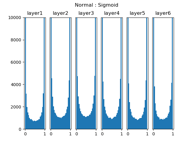
上图是一个 6层的深度网络，使用 全连接层 + Sigmoid 激活函数的配置，图中表示的是各层激活函数的直方图。可以看到各层的激活值严重向两侧 \([0,1]\) 靠近，从 Sigmoid 的函数曲线可以知道这些值的导数趋近于 0（激活函数值趋近于零，导数也趋近于零），反向传播时的梯度逐步消失。处于中间地段的值比较少，对参数学习非常不利。

传统的固定方差的高斯分布初始化方法，在网络变深的时候会使得模型很难收敛。

2.3，Xavier 初始化

基于上述观察（标准初始化在 Sigmoid 激活函数上的表现），Xavier Glorot 等人于 2010 年研究出了下面的Xavier 初始化方法。

Xavier 初始化方法比直接用高斯分布进行初始化 \(W\) 的优势在于：一般的神经网络在前向传播时神经元输出值的方差会不断增大，而使用 Xavier 等方法理论上可以保证每层神经元输入输出数据分布方差一致（和 BN 层效果类似，具体原理参考Xavier 论文）。

条件：正向传播时，激活值的方差保持不变；反向传播时，关于状态值的梯度的方差保持不变。

使用 Sigmoid 激活函数时，Xavier 高斯分布初始化的公式如下所示:

\[W \sim N \begin{pmatrix} 0, \sqrt{\frac{2}{n_{in} + n_{out}}} \end{pmatrix}\]

Pytorch 框架中对应的 API 如下。

torch.nn.init.xavier_normal_(tensor, gain=1)

另外，还有 Xavier 均匀分布的公式如下所示（个人感觉使用频率不多）。

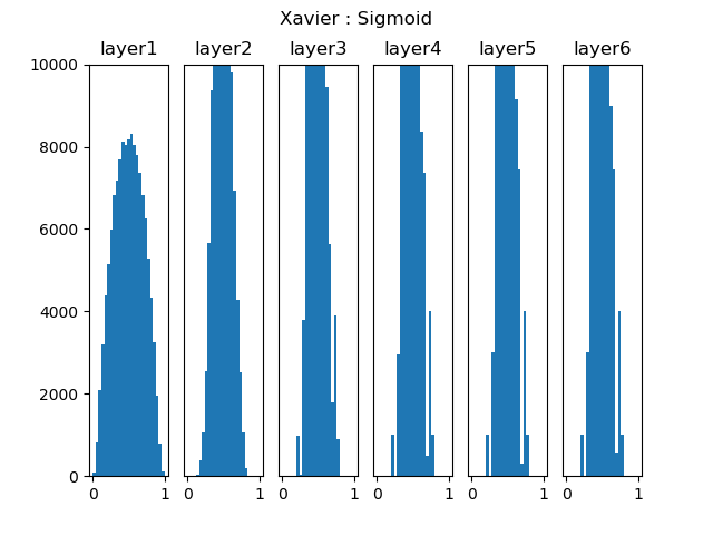
\[W \sim U \begin{pmatrix} -\sqrt{\frac{6}{n_{in} + n_{out}}}, \sqrt{\frac{6}{n_{in} + n_{out}}} \end{pmatrix}\]

下图2展示了 Xavier 初始化在 Sigmoid 激活函数上的表现，其和图1都基于同一个深度为 6 层的网络。可以看到，后面几层的激活函数输出值的分布仍然基本符合正态分布，这有利于神经网络的学习。

2.4，He 初始化

随着深度学习的发展，人们觉得 Sigmoid 激活在反向传播算法中效果有限且会导致梯度消失问题，于是又提出了 ReLU 激活函数。

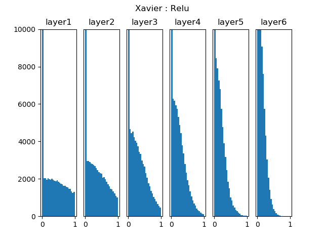
但 Xavier 初始化在 ReLU 激活函数上的表现并不好。随着网络层的加深，使用 ReLU 时激活值逐步向 0 偏向，这同样会导致梯度消失问题。

下图3展现了 Xavier 初始化在 ReLU 激活函数上的表现。

于是 He Kaiming 等人于 2015 年提出了 He 初始化法（也叫做MSRA初始化法）。

He 初始化法最主要是想解决使用 ReLU 激活函数后，方差会发生变化的问题。

只考虑输入个数时，He 初始化是一个均值为 0，方差为 \(2/n\) 的高斯分布，适合于 ReLU 激活函数:

\[W \sim N \begin{pmatrix} 0, \sqrt{\frac{2}{n}} \end{pmatrix}\]

其中 \(n\) 为网络层输入神经元数量个数。

Pytorch 框架中对应的 API 如下。

torch.nn.init.kaiming_normal_(tensor, a=0, mode='fan_in', nonlinearity='leaky_relu')

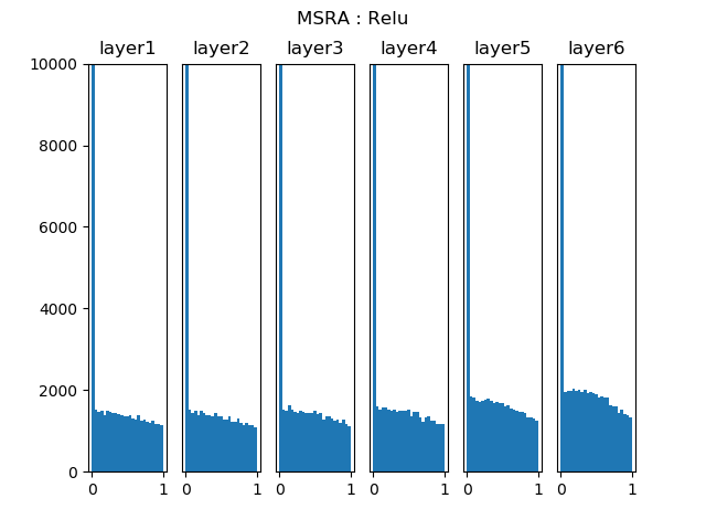
下图4 为 He 初始化在 ReLU 激活函数上的表现，所用网络和前面一样。

2.5，总结

• Xavier 初始化和 He 初始化目的都是想可以根据神经元连接数量自适应调整初始化分布的方差，也称为“方差缩放”。
• 网络参数初始化方法的选择对保持数值稳定性至关重要，其与非线性激活函数的选择得结合一起考虑。
• 网络参数初始化的选择可以决定优化算法收敛的速度有多快。糟糕选择可能会导致我们在训练神经网络模型时遇到梯度爆炸或梯度消失。

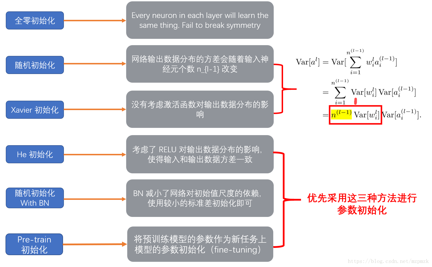
除了以上初始化，比较常用的还有“随机初始化 With BN”和“预训练模型初始化”，各种初始化方法的特点总结如下:

1. Overview of Parameter Initialization

Neural network models generally rely on the stochastic gradient descent optimizer to update their parameters, and parameter learning is a non-convex problem. When optimizing with gradient descent, the choice of the initial weight values is critical.

First, it should be clear that modern weight initialization strategies are simple and heuristic. Designing an improved initialization strategy is a difficult task, because neural network optimization is still not well understood (that is, model training is a black box).

Most initialization strategies aim to establish some nice properties at the moment of initialization. However, we do not understand well which of these properties are preserved, and under what circumstances, once learning begins. A further difficulty is that some initial points may be favorable from an optimization point of view yet unfavorable from a generalization point of view. Our understanding of how the initial point affects generalization is quite primitive and provides almost no guidance on how to choose it.

1.1 Why Network Parameters Need Initialization

The training algorithms of deep learning models (neural network models) are usually iterative, so the trainer must specify the starting point of the iterations — that is, choose a network parameter initialization strategy.

1.2 Why Network Parameter Initialization Matters

Training a deep learning model is hard enough that most algorithms are strongly influenced by the network initialization strategy.

The starting point of the iterations can determine whether the algorithm converges. Some initial points are so unstable that the algorithm runs into numerical difficulties and may fail completely. When learning does converge, the initial point can determine how fast it converges and whether it converges to a point with high or low cost. In addition, iterative points with the same loss cost may still have vastly different generalization errors, so the initial point can also affect generalization (error).

2. Classification of Weight Initialization Methods

In practice, initializing model weights from a Gaussian distribution or a uniform distribution are both effective approaches. Note that the difference between choosing these two distributions has not yet been studied in detail; what can be established is that the scale of the initial distribution strongly affects both the outcome of the optimization process and the generalization ability of the network.

Both the random values and the distribution used by a weight initialization strategy affect model performance, yet the underlying principle (the principle of neural network optimization) has not been thoroughly studied. Model training really does deserve its nickname of alchemy — sometimes it depends on the experience of the alchemist.

Another way to summarize neural network parameter initialization strategies is as follows:

1. Loading pretrained model parameters: directly load parameters trained on a large-scale dataset, which improves the model’s generalization ability to some extent.
2. Random initialization: note that parameters must not all be initialized to 0. If all hidden-layer activations are identical in the first forward pass, the weight updates in backpropagation are identical too, so the hidden neurons become indistinguishable — the “symmetric weights” phenomenon. A better approach is to randomly initialize every parameter.
3. Fixed-value initialization: for example, biases are usually initialized to 0; the forget-gate bias of an LSTM is usually set to 1 or 2 to enlarge gradients along the time axis; for ReLU neurons the bias is set to 0.01 so that they are easier to activate early in training.

Since different articles classify initialization methods differently, this article lists the commonly used and effective methods directly, together with the corresponding API in the PyTorch framework.

2.1 All-Zero Initialization

Although parameters (weights) should ideally stay roughly half positive and half negative (expectation 0), this does not mean that all parameters can be initialized to 0 (\(W=0\))! A printout of a weight matrix initialized to zeros looks like this:

W1= [[-0.82452497 -0.82452497 -0.82452497]]
B1= [[-0.01143752 -0.01143752 -0.01143752]]
W2= [[-0.68583865]
     [-0.68583865]
     [-0.68583865]]
B2= [[0.68359678]] # two-layer neural network with a single output

You can see that the three units inside W1, B1, W2 all hold identical values. Because the initial values are all zero, gradients are propagated back uniformly, so the weights W of all neurons are updated identically and never differentiate. No matter how many epochs are trained, the result will not be correct.

2.2 Standard Initialization

1. Gaussian initialization: initialize every parameter randomly from a Gaussian distribution, that is, initialize the weights \(W\) as follows:

\[W \sim N[0, \sigma^2]\]

Here \(N\) denotes the Gaussian distribution (also called the normal distribution). The formula above is a Gaussian distribution with location parameter \(\mu = 0\) (mean) and scale parameter \(\sigma^2\) (variance) — that is, the standard Gaussian distribution. Some sources also call it Normal initialization.

The corresponding API in the PyTorch framework is:

# By default the standard Gaussian initialization is used, i.e. mean 0 and variance 1
torch.nn.init.normal_(tensor, mean=0, std=1)

1. Similar to Gaussian initialization is uniform initialization, whose parameter range is \([-r, r]\).

The corresponding API in the PyTorch framework is:

torch.nn.init.uniform_(tensor, a=0, b=1)

Gaussian and uniform initialization are both methods with a fixed variance parameter, and the key question for both is: how should the variance be set?

• Too small: neuron outputs become too small, and the gradient signal disappears after several layers.
• Too large: the sigmoid gradient approaches 0, causing vanishing gradients. Usually this needs to be combined with a BN layer.

When the target problem is relatively simple and the network is not deep, standard initialization is usually sufficient. But with deep neural networks, standard initialization combined with the Sigmoid activation runs into the problem shown in Figure 1 below.

The figure above shows a 6-layer deep network configured with fully connected layers + Sigmoid activation; it presents histograms of the activations of each layer. The activations of every layer crowd heavily toward the two extremes of \([0,1]\). As the Sigmoid curve shows, the derivatives at these values approach 0 (as the activation approaches zero, so does its derivative), so gradients vanish progressively during backpropagation. Few values lie in the middle region, which is very unfavorable for parameter learning.

The traditional fixed-variance Gaussian initialization makes the model very difficult to converge as the network gets deeper.

2.3 Xavier Initialization

Based on the observation above (standard initialization with the Sigmoid activation), Xavier Glorot et al. developed the Xavier initialization method in 2010.

The advantage of Xavier initialization over initializing \(W\) directly from a Gaussian is that, whereas in an ordinary network the variance of neuron output values keeps growing during the forward pass, methods such as Xavier can theoretically guarantee that the variance of the input and output data distributions of each layer stays consistent (similar in effect to a BN layer; see the Xavier paper for the details).

Conditions: during the forward pass, the variance of the activation values stays unchanged; during the backward pass, the variance of the gradients with respect to the state values stays unchanged.

For the Sigmoid activation, the formula for Xavier Gaussian initialization is:

\[W \sim N \begin{pmatrix} 0, \sqrt{\frac{2}{n_{in} + n_{out}}} \end{pmatrix}\]

The corresponding API in the PyTorch framework is:

torch.nn.init.xavier_normal_(tensor, gain=1)

In addition, the formula for Xavier uniform initialization is shown below (in my experience it is not used very often).

\[W \sim U \begin{pmatrix} -\sqrt{\frac{6}{n_{in} + n_{out}}}, \sqrt{\frac{6}{n_{in} + n_{out}}} \end{pmatrix}\]

Figure 2 shows Xavier initialization with the Sigmoid activation; it is based on the same 6-layer network as Figure 1. As you can see, the distribution of the activation output values in the later layers still roughly follows a normal distribution, which is beneficial for learning.

2.4 He Initialization

As deep learning developed, Sigmoid activation came to be regarded as limited in backpropagation and prone to vanishing gradients, so the ReLU activation was proposed.

However, Xavier initialization does not perform well with the ReLU activation. As network layers get deeper, activation values under ReLU gradually shift toward 0, which again leads to vanishing gradients.

Figure 3 shows Xavier initialization with the ReLU activation.

He Kaiming et al. therefore proposed He initialization (also called MSRA initialization) in 2015.

He initialization mainly aims to solve the change in variance caused by the ReLU activation.

Considering only the number of inputs, He initialization is a Gaussian distribution with mean 0 and variance \(2/n\), suitable for the ReLU activation:

\[W \sim N \begin{pmatrix} 0, \sqrt{\frac{2}{n}} \end{pmatrix}\]

where \(n\) is the number of input neurons of the layer.

The corresponding API in the PyTorch framework is:

torch.nn.init.kaiming_normal_(tensor, a=0, mode='fan_in', nonlinearity='leaky_relu')

Figure 4 shows He initialization with the ReLU activation, using the same network as before.

2.5 Summary

• Both Xavier and He initialization aim to adapt the variance of the initialization distribution to the number of neuron connections, which is also called “variance scaling”.
• The choice of initialization method is essential for maintaining numerical stability, and it must be considered together with the choice of nonlinear activation function.
• The choice of initialization can determine how fast the optimizer converges. A poor choice may leave us facing exploding or vanishing gradients while training the network.

Besides the methods above, “random initialization with BN” and “pretrained model initialization” are also common. The characteristics of the various initialization methods are summarized below: